How To Scale
While there are already excellent posts on scaling, I wanted to share my own understanding and things i've learned from my past few months and hopefully spark some discussion. I hope this post can shed light for anyone navigating the challenges of scaling up neural networks. And there may be mistakes or inaccuracies, so if you want to correct me or would like to discuss further, please feel free to DM me on X or leave a comment.
Last Update: Dec 31st 2025
Before we dive in, I’d like to acknowledge that this post is heavily inspired by Simo Ryu’s “What to do to scale up?”, and the post theme is based on diffusionflow.github.io by GDM.
Motivation
"how to scale" in this post means “how we should set the initialization standard deviation (init std), learning rate (lr), and batch size (bsz) and other hyperparameters (HPs) as model size (including both width and depth) and dataset size grow”. It is so true that as you scale up computing budget, \(C=6ND\) (where \(N\) is model size and \(D\) is dataset size), your model tends to perform better.
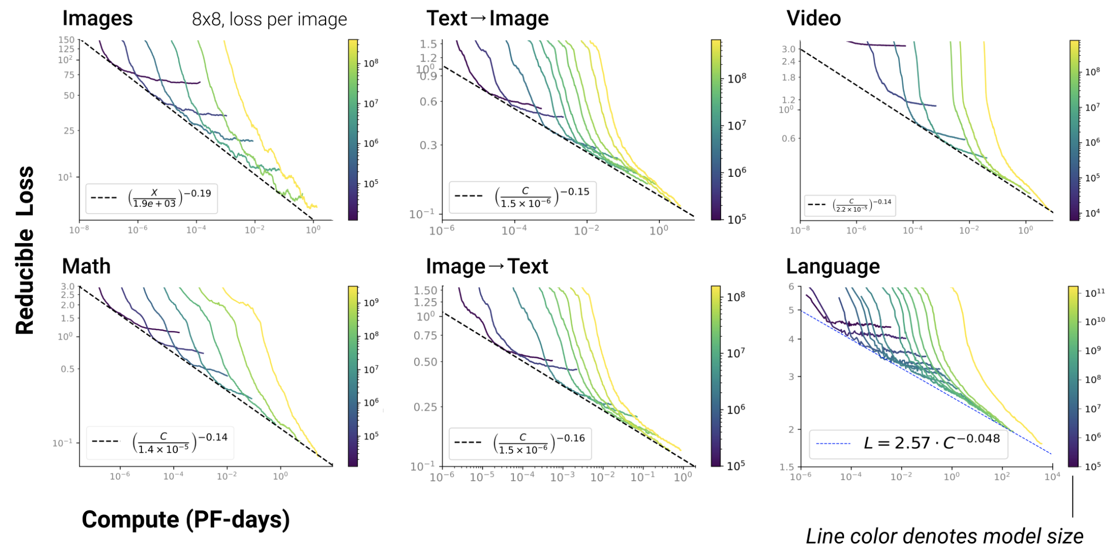 Fig. Scaling Law is Universal Behavior. For Every Tasks, It Works. Source from Scaling Laws for Neural Language Models
However, scaling law papers never tell us how to set the lr or bsz for a given computing budget, C. This is a non-trivial issue, because “more compute always leads to better performance” is not guaranteed unless you’re using near-optimal HPs for each \(C\).
If you fail to find the right HPs, you might conclude:
“WTF? larger isn’t better? okay, let’s quit scaling.”
and you're not gonna make it.
That’s exactly why we need to understand “how to scale.”
So, the main questions we should know are:
- How should the lr be scaled with compute budget \(C\)?
- How should optimal or critical bsz be scaled with \(C\)?
- Alternatively, how should lr and bsz be scaled individually with \(N\) or \(D\)?
From the perspective of model size, there is a theoretically grounded method for ensuring optimal lr transfer across different scales. It’s called Maximal Update Parameterization (muP). You’ve probably heard about it on X (formerly twitter).
Compared to muP, Standard Parameterization (SP) (e.g. He, Lecun, and other default PyTorch initializations) is not designed for scaling.
These methods are well-defined only at initialization, not during training.
That means they don’t account for how weight updates affect model behavior and it finally leads to what’s known as “left-shifted lr curves”. But we don’t want to this shifting trends. Our goal is to define a parameterization in which optimal behavior transfers as model size scales. That means we need to properly set per-layer:
- lr
- init std
- multiplier
And by anaylzing optimization behavior carefully, muP finally give us right parameterization to scale up model size properly.
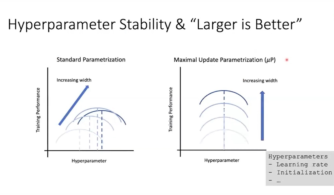 Fig. Source from Greg Yang’s Video
What really matters isn’t something like:
“For the 8B model, optimal lr is 3e-4; for 405B it’s 8e-5.”
Rather, it’s:
“The optimal lr at 40M is 0.00195, so we should halve the lr when we double the width (hidden size).”
If we define this scaling rule properly, we can efficiently tune larger models, and match scaling laws, at relatively low cost.
The authors of Tensor Program (TP)-V, aka muTransfer, Greg Yang and Edward Hu, were part of the early OpenAI–Microsoft collaboration. Andrew Carr, formerly at OpenAI, confirmed that muP was likely used in training GPT. (GPT-4 technical report also refers to TP-V)

 Fig. Source tweet
Note that, even this elegant muP framework does not consider dataset scaling. We’ll discuss this point later in the post.
How to Scale Model Size (Parameterization, ...)
Maximal Update Parameterization (muP) (What 'Maximal' actually means?)
It’s important to note that muP literally stands for Maximal Update.
Many people often misunderstand muP is only about hyperparameter (HP) transfer, but that’s not true.
Of course, HP transfer is a nice property. it allows us to avoid extensive grid searches over HPs for a given compute budget \(C\) when predicting scaling laws or training very large models.
But muP is fundamentally about ensuring that every layer learns features maximally at each optimization step, by assigning per-parameter HPs (lr, init std, etc.), even as the network’s width goes to infinity.
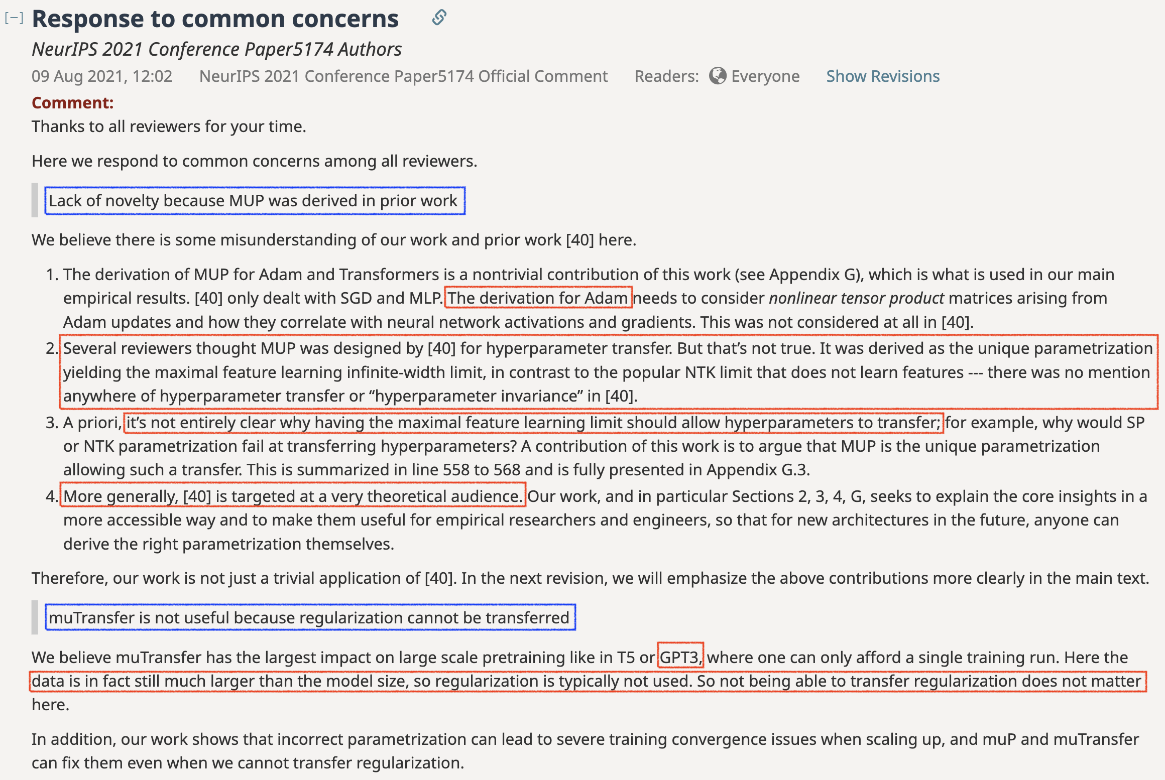 Fig. Openreview of TP-V. Greg Yang explain ‘muP is not only for HP transfer’
So, muP is designed to enable maximal feature learning, but Why SP is not enough? In SP, we often find that some weights receive disproportionately large gradients, while others receive gradients that are too small.
If we reduce the lr to stabilize the weights that receive large gradients, the others can become stuck meaning they don’t learn enough features, which leads to inefficient training.
On the other hand, if we increase the lr too much, the model may diverge. So we are in the dilemma.
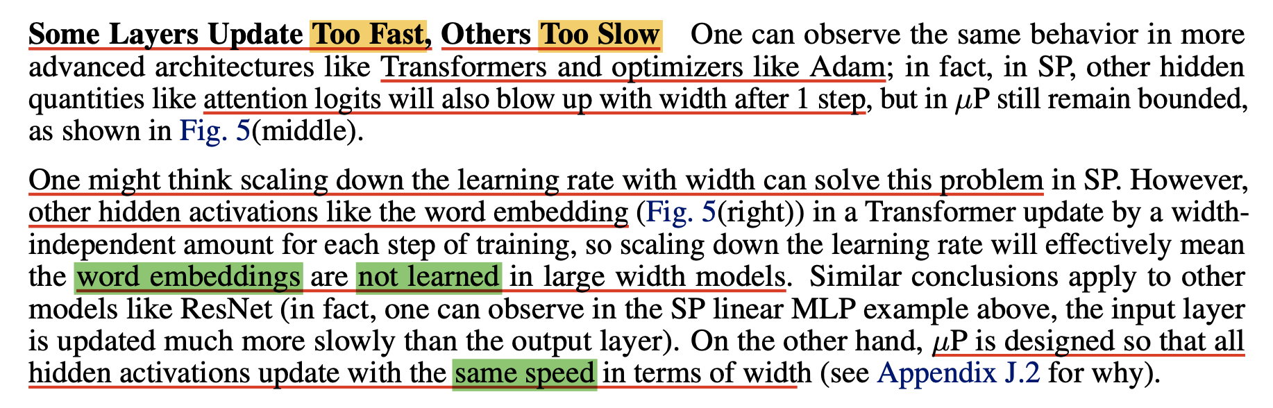 Fig. In TP-V paper, it is clearly mentioned.
That’s why we need to carefully analyze ‘per-layer behavior’ and adopt ‘per-layer parameterization (i.e., per-layer lr, init std, and multiplier)`, as done in muP.
Of course, there may be other viable approaches.
Normalization techniques such as BatchNorm and LayerNorm can help correct imbalances and improve optimization.
Adaptive optimizers may also help, but normalization and Adam alone are insufficient.
Recently proposed advanced optimizers like Muon (with proper scaling factors) and SCION show that lr can transfer across model widths. (i’ll cover this later in this post)
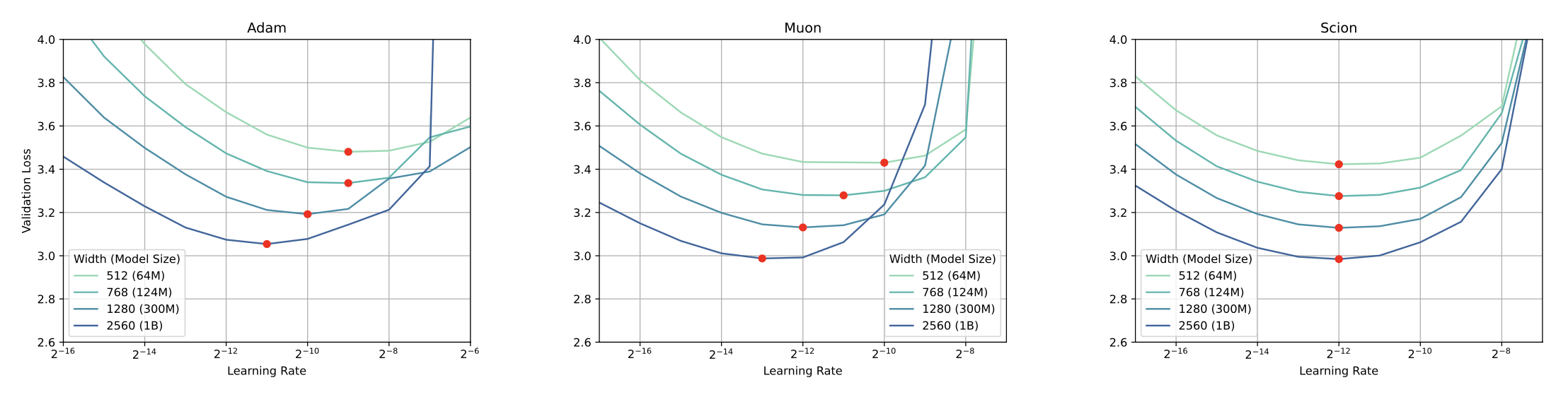 Fig. Source from Training Deep Learning Models with Norm-Constrained LMOs. lr can be transferred with SCION optimizer
IMO, most optimization and training techniques share the same motivation: to stabilize, balance, and improve training dynamics, seen from a unified perspective.
Anyway, muP is based on three core desiderata:
- Training stability (pre-activation should not be blown up when model’s width is scaled up)
- Feature learning (feature should be changed enough)
- Non-triviality (weight should not be stuck at initialization)
By solving for these desiderata, you get a parameterization that not only encourages maximal feature learning but also theoretically guarantees HP transfer across width. (Again, i’d like to say HP transfer was never the primary goal. it follows)
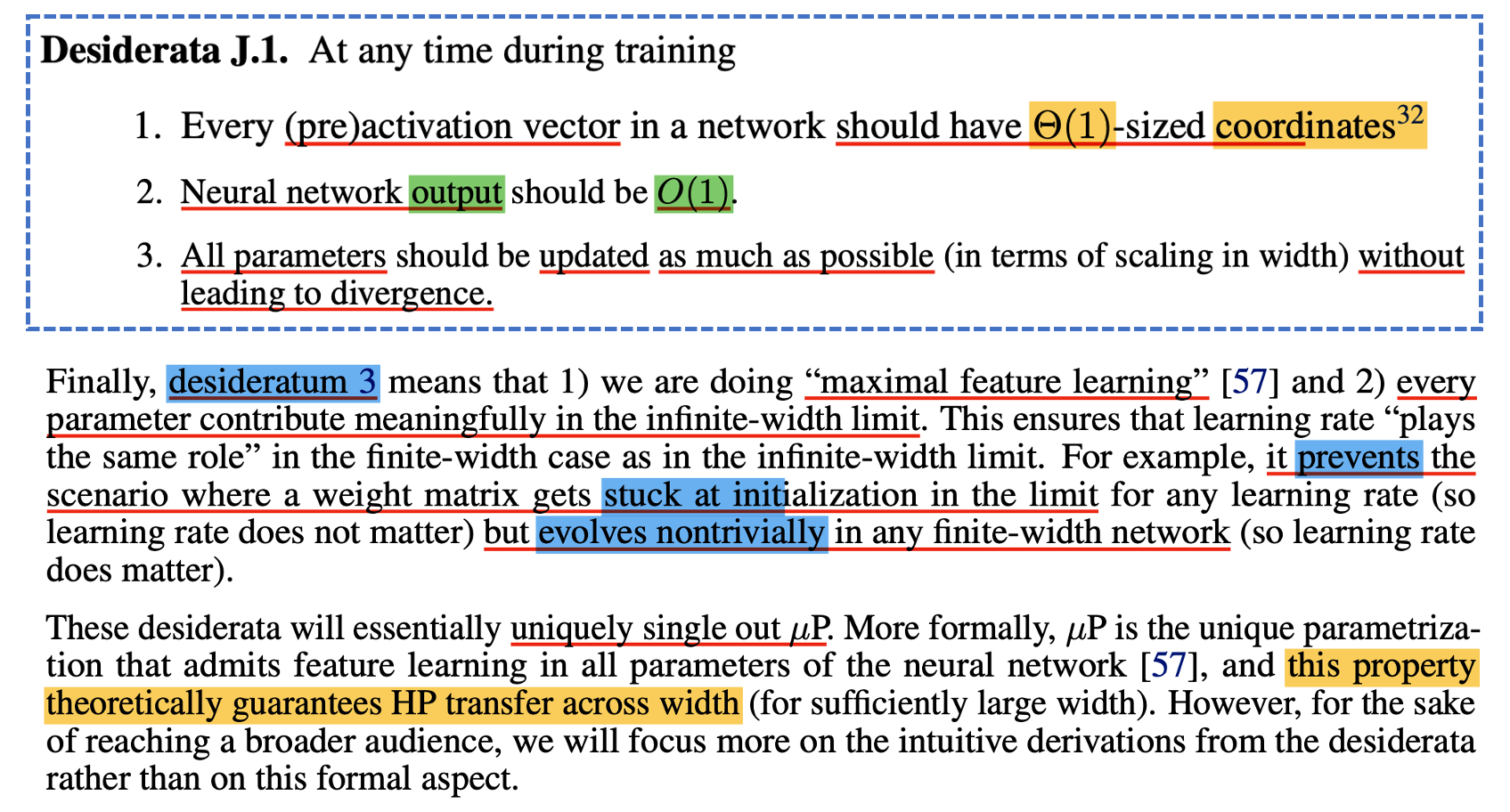
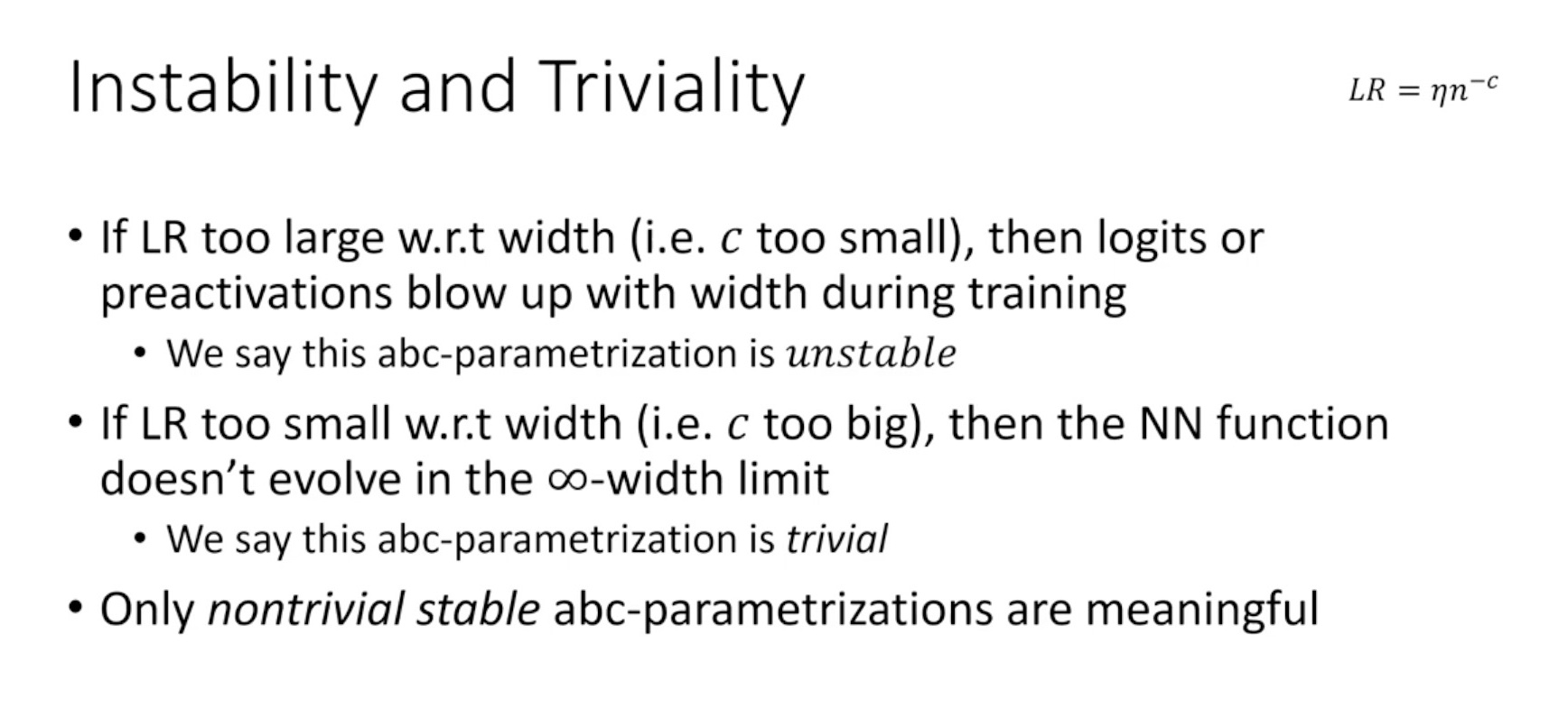
Why does training stability matter?
Because muP is a method for feature learning in the infinite-width regime, where hidden sizes grow larger and larger (e.g., 1024, 4096, …, 40k).
This means muP must ensure maximal learning regardless of width, so we don’t want pre-activations to scale with the width \(n\).
That’s why muP enables training dynamics to be transferred across different model scales.
Of course, there are many other parameterizations, such as Standard Parameterization (SP), Neural Tangent Kernel (NTK), Mean Field Theory (MFT) and muP. One might ask, “Why is muP unique for maximal feature learning?”
I won’t go into full detail here, check the original paper, but consider this:
In the kernel regime (e.g., NTK), models are effectively frozen in feature space.
So even if your NTK-parameterized BERT is pretrained successfully, its learned representation is weak.
Assume you tried to concatenate a randomly initialized linear layer to its hidden features and fine-tune.
If the model trained with NTK parameterization, it wouldn’t work well because the hidden layers never learned meaningful features even though it’s pretrained performance is not bad. That’s the problem and muP doesnt want to allow this.
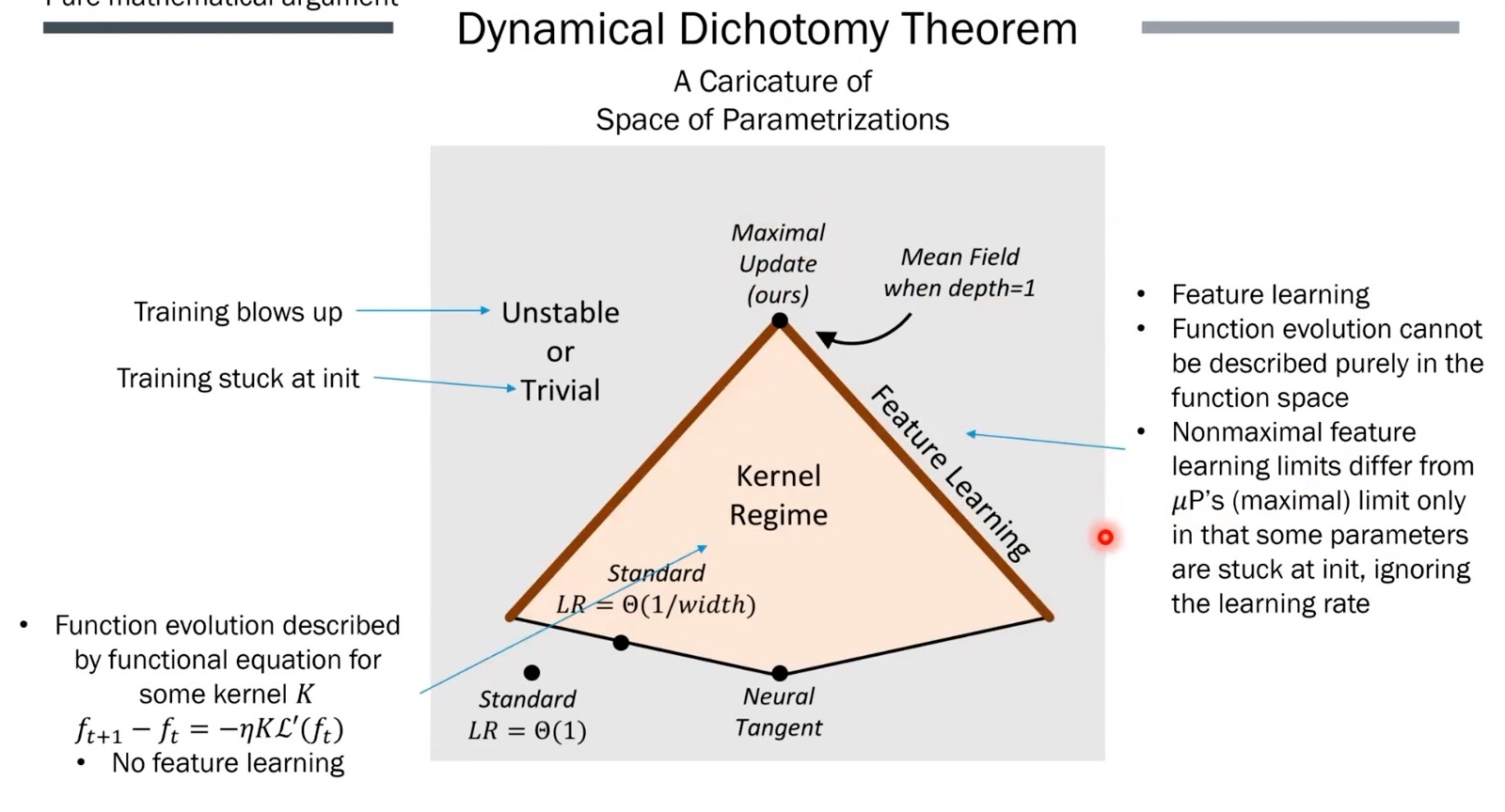 Fig. The caricature provided in paper might not be intuitive, but what authors want to say is that among other paramterizations, only muP allows stable, non-trivial feature learning. some (NTK) are stuck in kernel regime and another (SP with large lr) diverges.
For more motivation (even though below example isn’t strictly about parameterization, but i’d like to raise the research question), transformers with pre-norm often show redundancy in deeper layers. Post-norm based transformer, which is originally proposed in Attention Is All You Need is better than Pre-norm variant at performance, but post-norm does not preserve upstream gradients (identity mapping), so it requires lr warmup stage or other tactics to improve training stability. However, for pre-norm it makes harder for the residual features in deeper layers to contribute to the model’s main residual stream, a phenomenon known as ‘representation collapse’ as a side-effect.
So in this case, feature learning across layers can become uneven, and it leads to waste of compute.
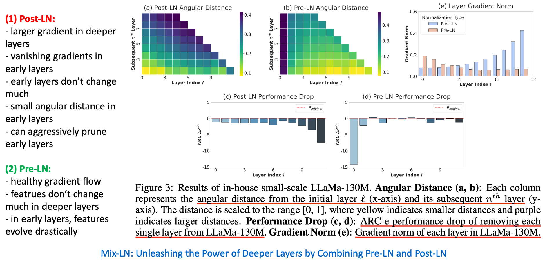
Many researchers studied normalization module or parameterization like residual post norm (sandwich norm), mix-ln, deep-norm, or depth scaled sandwich norm, … to achieve both training stability, and effective feature learning.
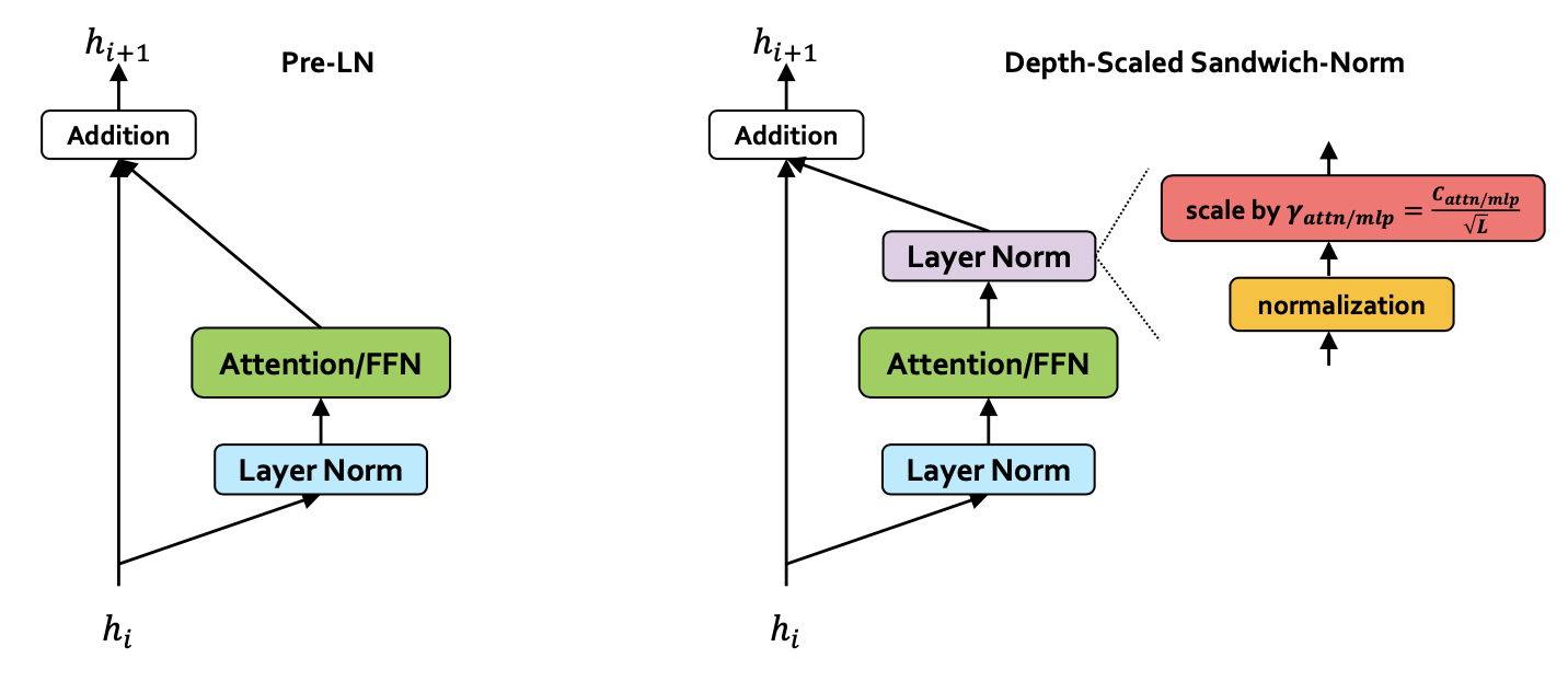 Fig. depth scaled sandwich norm from Pangu Ultra
IMO, i believe these examples are related to parameterization too.
In TP-V, the authors show that muP not only transfers optimal lr across width,
but also achieves better performance overall in Language Modeling (LM) task (GPT-3 setup).
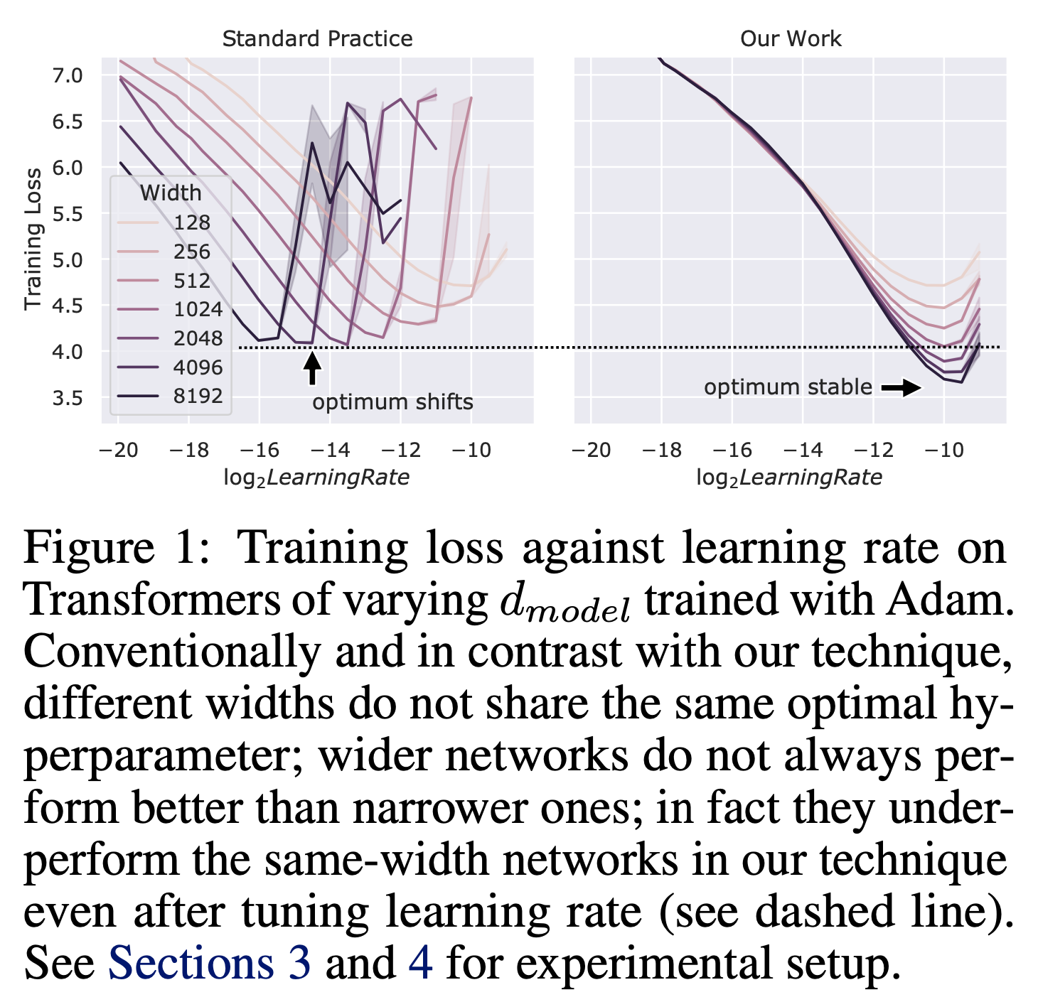 Fig. muP not even transfrer optimal lr but also show better performance.
 "wider is always better"
That said, in real-world scenarios, maybe it’s not true that muP always outperform SP. In my own experience, muP has shown stronger benchmark results at small to medium scales (e.g., 200–300B tokens),
but the returns seem to diminish as scale increases. my guess is that even though other parameterizations such as SP is in the lazy training regime,
the embedding and output layers eventually start learn something in later. (or maybe… it’s just my skill issue)
Key Intuition and Derivation of muP
Now we’re gonna derive unique scaling rule for maximal update and HP transfer.
Before diving into muP, let’s briefly review Standard Parameterization (SP). SP focuses on initialization. But what defines ‘good’ at initialization?
- The goal is to prevent gradient explosion or vanishing.
- Since gradient signal for Neural Network (NN) training is derived by backpropagation (chainrule), we want pre-activations to stay around unit scale.
 Fig. Source from Sergey Levine’s ML Lecture (CS182)
Assume weight matrix is i.i.d sampled from normal distribution and input feature of this layer is also i.i.d. In forward propagation, the output pre-activations of this layer, \(z=Wx \in \mathbb{R}^{\text{fan-out} \times 1}\)’s elements have \(\text{fan-in} \cdot \color{red}{\sigma_W^2}\) variance if \(x \in \mathbb{R}^{\text{fan-in} \times 1} \sim \mathcal{N}(0,1)\) (it is fair assumption because we typically standardize inputs of each modules), and \(W \in \mathbb{R}^{\text{fan-out} \times \text{fan-in}} \sim \mathcal{N}(0,\sigma_W^2)\).
\[\begin{aligned} & z_i = \sum_j^{\text{fan-in}} W_{ij} x_j & \text{no bias }\\ & \mathbb{E}[z_i^2] = \sum_j^{\text{fan-in}} \mathbb{E}[W_{ij}^2] \mathbb{E}[x_j^2] = \text{fan-in} \cdot \color{red}{\sigma_W^2} \cdot \sigma_x^2 & \\ \end{aligned}\]To keep this around 1, we should counter this value by \(\text{fan-in}\). And this is why SP is called fan-in (input feature dim) variance.
It means every element (coordinate) of weight matrix has roughly \(1/\text{fan-in}\) size value.
Also, there is a lot of init method like Xavier Init, He Init and so on. Especially, for Xavier Init, it consider backpropagation at initalization point. Because \(dL/dx\) is outer product of upstream gradient and weight matrix, we can derive backward propagation similar to forward, \(dL/dx \sim \mathcal{N}(0, \text{fan-out}\sigma_W^2 \sigma_x^2)\). If matrix shape is \(n \times n\), Xavier is same as Lecun init.
 Fig.
Fig.
Howerver, as i mentioned, SP is only for initilziation. What we want is every (pre-)activations has constant scale (\(\Theta(1)\)) at any time in training step, regardless of the hidden size of neural network.
In Tensor Program (TP) (muP is from TP-4 and 5), It does not only care initialization but also training dynamics. This is why muP is called mu + Paramtereization. Parameterization includes all three thing, per parameter 1) initialization (init std), 2) multiplier, 3) learning rate (lr) but SP only describe initialization standard deviation (init std).
Again, for deriving muP, you should remember muP’s three desideratums. We just want our model to act like this.
 Fig.
Fig.
However, once you try to derive muP, it could be overwhelming because of too many mathematical symbols.
But don’t worry, because in this post, we’ll derive muP as if we had no brain, keeping things as simple as possible. All you need is Law of Large Numbers (LLN), Central Limit Theorem (CLT), a bit of intuition about SGD and Adam, and the important fact that Neural Network (NN) training is indeed just bunch of dot products (forward pass) and outer products (backward pass). (I’m not going to derive muP very strictly in this post because it’s mathematically heavy.)
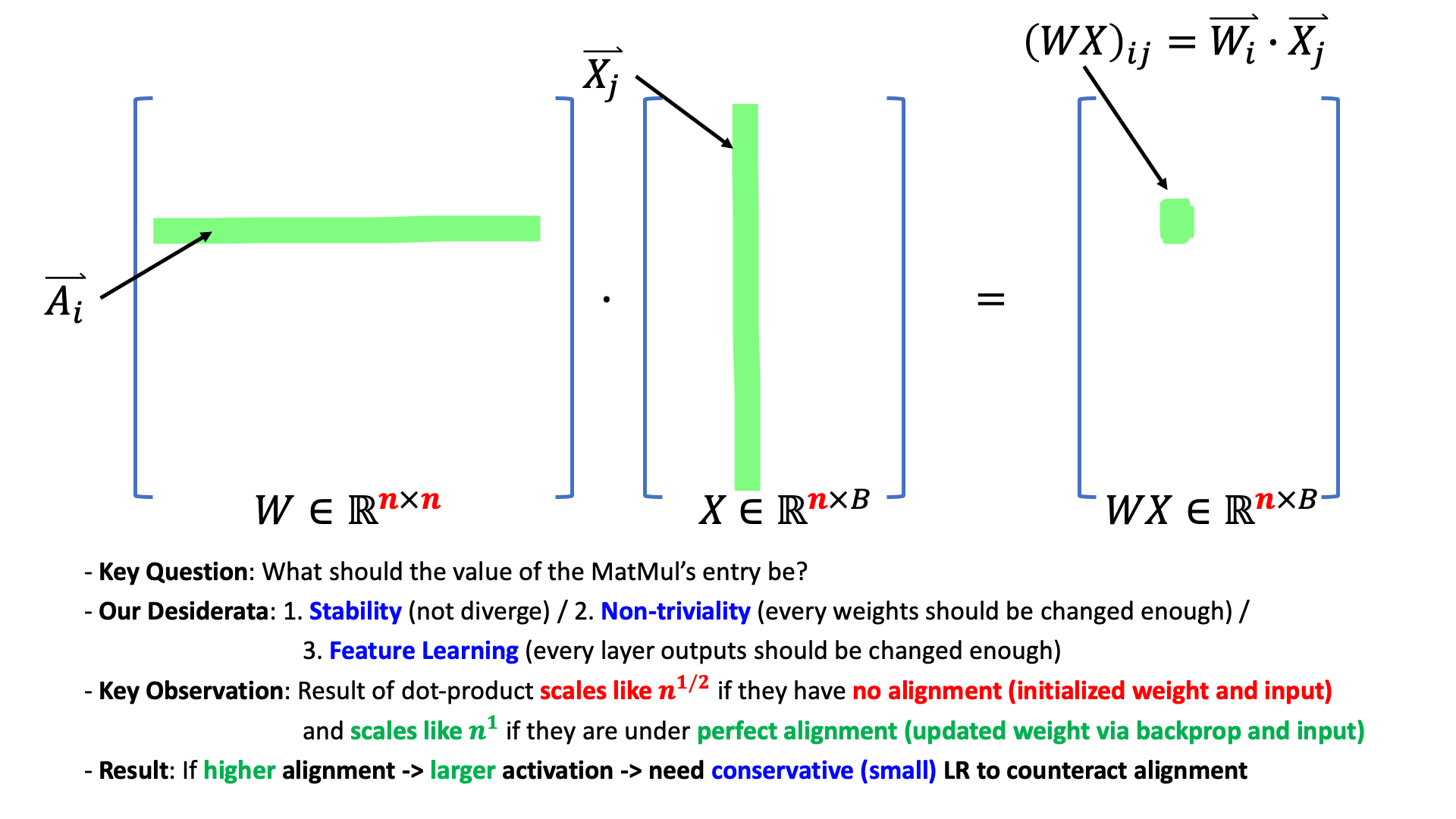 Fig.
Fig.
Typically, dot product of n-dimensional vectors get larger when width, n goes to infinity (we should counter this behavior). The key rule of muP is as follows.
- each element’s scale of output vector is the dot product result of n-dimensional vectors
- if these vectors are correlated (aligned, similar direction) it’s output value follows LLN.
- so you should counter this behavior by \(n\)
- if they are not correlated (like i.i.d at init point), it follows CLT.
- so you should counter by \(sqrt(n)\)
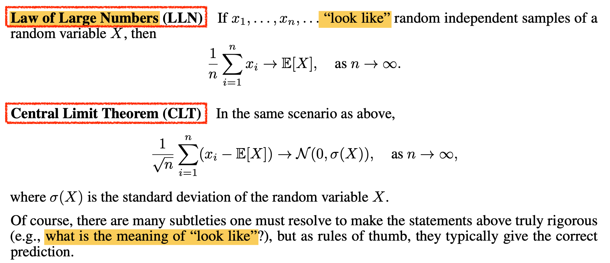 Fig. TP-V
To understand muP, let’s say at \(t\) step’s weight matrix is \(W_{t} \in \mathbb{R}^{n \times n}\), input \(x \in \mathbb{R}^{n \times 1}\) and it’s output pre-activation, \(z_t \in \mathbb{R}^{n \times 1}\). So, the output pre-activation at initialization step (\(t == 0\)) is as follows
\[z_0 = \underbrace{W_{0} x}_{\Theta(1)}, W_0 \sim \underbrace{\mathcal{N}(0, (\frac{1}{\sqrt{n}})^2)}_{\text{like SP}}\]For the forward pass, we don’t want the output to blow up with width. That means we want to preserve pre-activation output as \(\Theta(1)\). Here \(\Theta(1)\) means output pre-activation’s scale does not depend on model width (embedding dim), \(n\). That is, muP is scale invariant (good behavior for HP transfer).
The symbols \(\Theta(\cdot)\) and \(O(\cdot)\) are known as asymptotic notations, commonly referred to as Big O notation. While widely used in CS to describe algorithmic complexity, they actually originate from mathematics (and Greg Yang comes from a mathematical background as far as i know). There are three asymtotic notation, and you’ll notice both \(O\) and \(\Theta\) are used for muP derivation.
- 1.\(O(\cdot)\): Upper bound – the function grows at most this fast.
- 2.\(\Omega(\cdot)\): Lower bound – the function grows at least this fast.
- 3.\(\Theta(\cdot)\): Tight bound – the function grows exactly this fast (within constant factors).
 Fig. Source from here
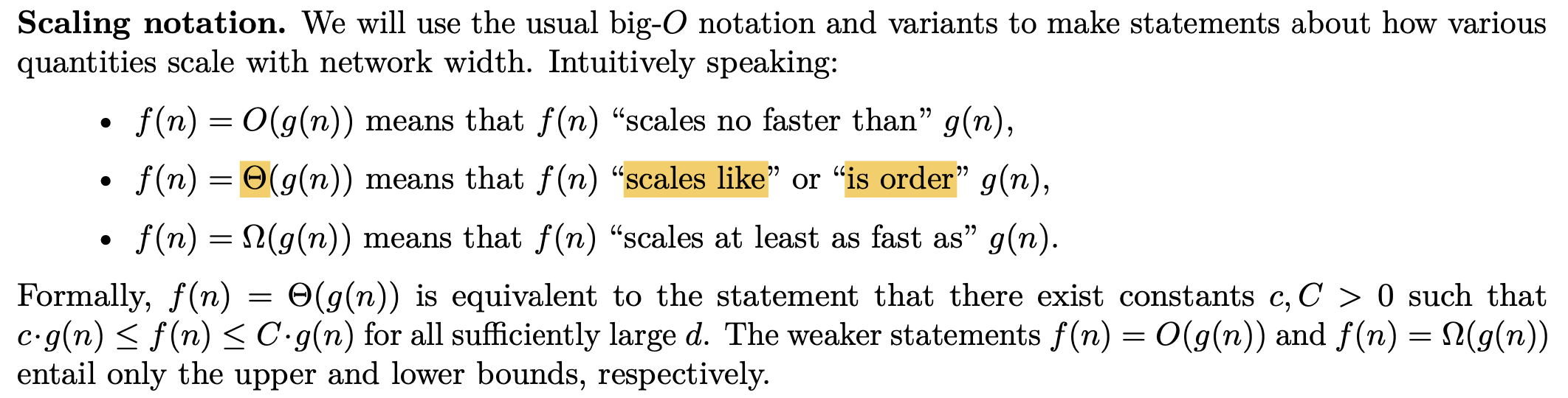 Fig. Source from A Spectral Condition for Feature Learning
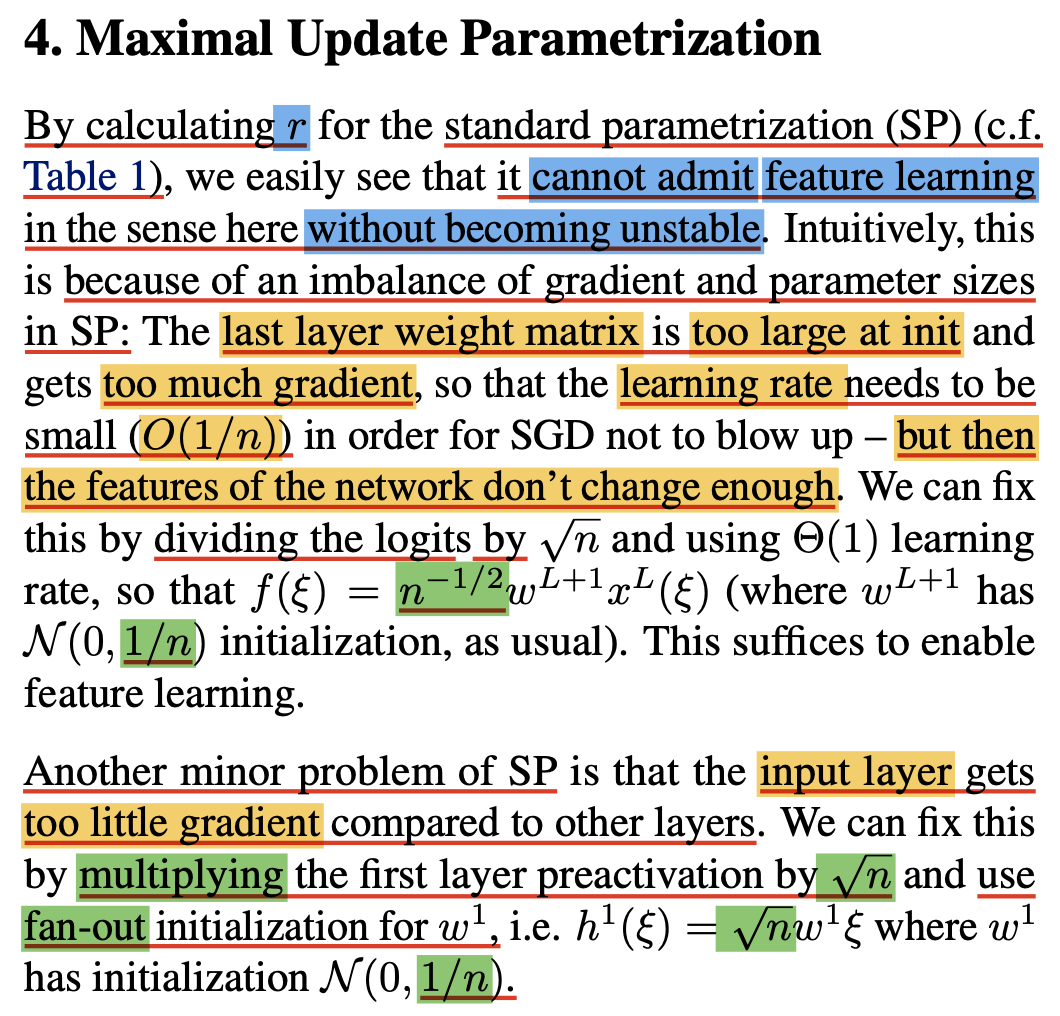
Anyway, we can just use fan-in variance (fan-in (featrue in) dim is n) like SP for forward stability at initilization. But after single optimization step (SGD or Adam; let’s assume SGD first), the weight is updated as:
where \(\eta\) is lr, and \(g_t\) is upstream gradient. Now \(t+1\) step’s pre-activation can be described as
\[\begin{aligned} & z_{t+1} = W_{t+1} x' & \\ & = (W_{t} + \eta \nabla_{W_{t}}L)x' & \\ & = W_t x' + \eta g_t (x^T x') & \\ \end{aligned}\]where \(x'\) is new input feature of \(t+1\) step and SP does not consider how \(\Delta W\) contributes \(t+1\) step’s pre-activation output at all. Dot product between column vector of weight matrix and input features are not correlated (they are i.i.d sampled) at the init point, but it start to be correlated after just one optimization step .
In above formula, we can reparameterize \((x^T x')\) term as \(n \cdot (x^T x')/n\) or \(\sqrt{n} (x^T x')/\sqrt{n}\), and these quantities, \((x^T x')/n\) or \((x^T x')/\sqrt{n}\) will be converged to some deterministic scalar following LLN or CLT as \(n\) goes to infinity. If \(x\) and \(x'\) are not correlated, it follows CLT, and if they are correlated, it follows LLN.
Why?
Let’s recap LLN and CLT briefly and think bout dot product of two vectors with 2 different conditiones, correlated or not. First, the Law of Large Numbers (LLN) is a basic concept in probability and statistics stating that the mean of \(n\) random samples converges to the mean as \(n\) becomes large (goes to infinity):
\[\frac{1}{n} \sum_{i=1}^n x_i \;\rightarrow\; \mathbb{E}[X], \quad\text{as } n \rightarrow \infty\]Here, each sample must be drawn independently from the same distribution, the “independent and identically distributed (i.i.d.)” assumption where it’s e.g. if you flip a fair coin 1,000 times, the outcome of the 550th flip does not depend on the results of the first 549 flips, and each flip follows the same \(\mathrm{Bernoulli}(1/2)\) distribution.
The Central Limit Theorem (CLT) is another convergence theorem for i.i.d. samples. It states that, for sufficiently large \(n\), the distribution of the sample mean of \(n\) draws approaches a normal distribution, regardless of the original distribution’s shape. Concretely, if you draw \(n\) samples from \(\mathcal{N}(\mu,\sigma^2)\), then the distribution of their mean,
\[\frac{1}{n}\sum_{i=1}^n x_i,\]converges to \(\mathcal{N}\bigl(\mu,\sigma^2/n\bigr)\). A common misconception is to think that CLT says “if you draw many samples, those individual samples become normally distributed,” but in fact CLT refers to the distribution of the sample mean, not the raw samples.
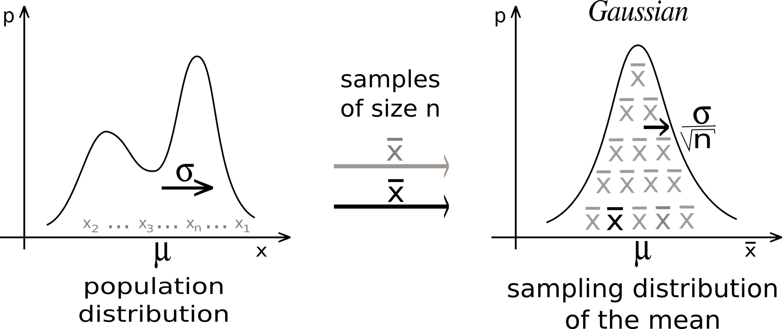
Fig. Source: Wikipedia
If we assume \(\mathbb{E}[x_i]=0\), CLT can be written more simply as
\[\begin{aligned} &\frac{1}{\sqrt{n}} \sum_{i=1}^n x_i \;\rightarrow\; \mathcal{N}(0,\sigma^2), \quad \text{as } n \rightarrow \infty,\\ &\text{where } \mathbb{E}[x_i^2] = \sigma^2. \end{aligned}\]More generally, then centering each sample by its mean,
\[\frac{1}{\sqrt{n}} \sum_{i=1}^n \bigl(x_i - \mathbb{E}[X]\bigr) \;\rightarrow\; \mathcal{N}(0,\sigma(X)^2), \quad \text{as } n \rightarrow \infty.\]And finally, we can write sum of i.i.d sample as follows
\[\begin{aligned} S_n =\sum_{i=1}^n x_i &= \underbrace{n\mu}_{\text{by LLN}} + \underbrace{\sqrt{n}\,\sigma\,\mathcal{N}(0,1)}_{\text{by CLT}} + \text{lower-order terms},\\ &\text{where } \mathbb{E}[x_i]=\mu,\;\mathbb{E}[x_i^2]=\sigma^2 \end{aligned}\]This is quite intuitive because one sample from \(\mathcal{N}(\mu,\sigma^2)\) will lie near \(\mu + \sigma\,\mathcal{N}(0,1)\), and \(\mathrm{Var}(X+Y) = \mathrm{Var}(X) + \mathrm{Var}(Y)\) if X, Y are independent and \(\mathrm{Var}(cX) = c^2\,\mathrm{Var}(X)\). in this form, if mean is non-zero, \(n\mu\) (from LLN) become dominant and if it’s zero, the next largest term, \(\sqrt{n}\sigma\,\mathcal{N}(0,1)\) (from CLT) become dominant.
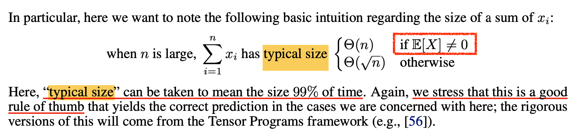 Fig. TP-V
We discuss about dot product of two vectors and it looks like
\[x^T x = \sum_{i=1}^n x_i x'_i = (x_1x'_1 + \cdots + x_nx'_n)\]Suppose if two vectors are correlated. In other words, if they are aligned, each elements’ mean value become non-zero, so it follows LLN. And intuitively, in large enough model scenario, typically each coordinate of \(x\) is i.i.d and \(x\) and \(x'\) are correlated even though they are mini-batch sampled, So \((x^T x')/n\) converges to some deterministic scalar by LLN.
\[\begin{aligned} & z_{t+1} = W_{t+1} x' & \\ & = (W_{t} + \eta \nabla_{W_{t}}L)x' & \\ & = W_t x' + (\color{red}{n} \eta) g_t \underbrace{ \frac{(x^T x')}{\color{red}{n}}}_{\text{deterministic scalar}=c} & \\ \end{aligned}\]and here deterministic scalar is \(c=\mathbb{E}Z^{x}Z^{x'}\) where \(Z^{x}, Z^{x'}\) are random variable of each vectors.
Hold on, what just happen?
By introducing \(n/n\) term, now we got \(n \times \eta\) term, and it means "if model width goes to infinity, the update quantity will be blown up", and we don’t want to allow this for stability. So, we should counter this behavior by \(n\).
However, it’s upstream gradient, \(g_t\) already consists of \(\Theta(1/n)\) scale entries, we don’t need to counter this in SGD optimizer setup. (simply put, gradient with respect to the output logit is \(\Theta(1)\) and weight matrix has \(\Theta(1/\sqrt{n})\) coordinate, but in muP, we divide output logit by \(\sqrt{n}\) or use \(\Theta(1/n)\) std. so we can think the upstream gradient \(g_t = W \otimes dL/dy\) can have typical size of \(\Theta(1/n)\). we will discuss this later in this post)
\[\begin{aligned} & z_{t+1} = W_{t+1} x' & \\ & = (W_{t} + \eta \nabla_{W_{t}}L)x' & \\ & = W_t x' + (\color{red}{n} \eta) \underbrace{g_t}_{\Theta(1/n)} \underbrace{ \frac{(x^T x')}{\color{red}{n}}}_{\text{c}} & \\ \end{aligned}\]But if we use adaptive optimizer like Adam, gradient is rescaled by elementwise, so, we should scale lr by \(1/n\) to explicitly counter. That’s why we can simply put “muP = 1/n lr rule for hidden layers (under Adam)”.
Actually, it’s more than CLT, LLN and dot product. we should consider full optimization trajectory with momentum and other factors. and bsz is greater than one in real world scenario where gradient is averaged by multiple rank 1 gradient and things go wild. if you want to see full derivation, i recommend you to read TP-IVb, TP-V or A Spectral Condition for Feature Learning. (Though i derive muP following original TP with LLN, CLT, I highly recommend Spectral Condition paper by Greg Yang, James B. Simonand Jeremy Berstein who is co-creater of Muon Optimizer)
Anyway, it’s all about CLT, LLN and dot product intuitively. Choose LLN or CLT based on whether the vectors are correlated or not. And this scaling logic holds for any dot product. That’s it.
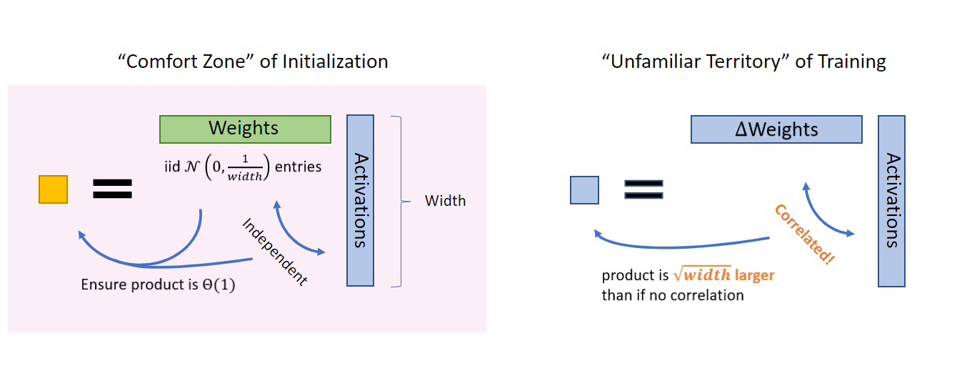 Fig. SP is only well defined at the initialization point (confort zone) but not during training. typically, if there is correlation, dot product become \(\sqrt{n}\) times larger than it’s not. Source from Greg Yang’s Blog
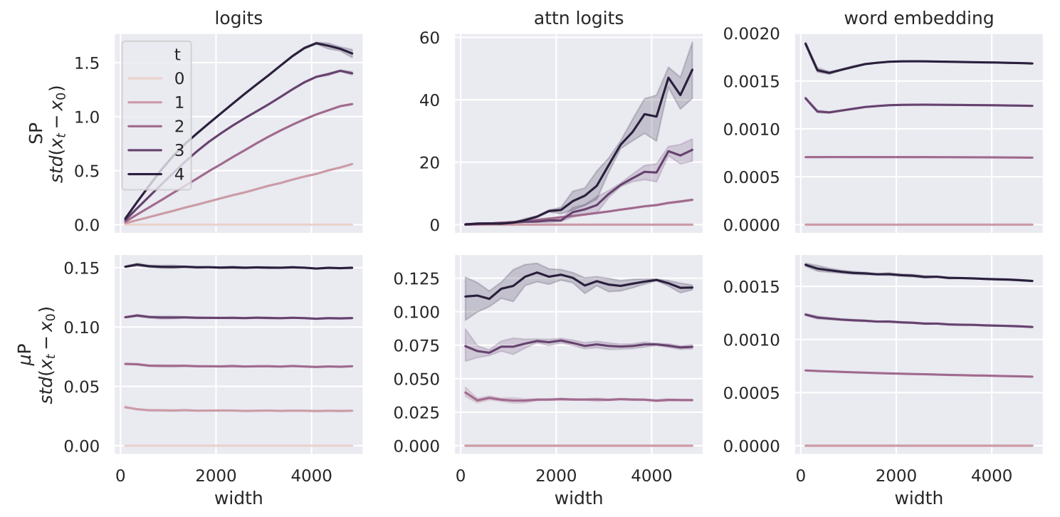
So, compared to SP, muP ensures every transformer module’s pre-activation don’t blow up in anytime during training times as n goes tends to infinity. Below figure is called coordinate check where coordinate means each element value of vector.

And now, one can accept it ensures maximal feature learning for every layers without instability, and all init std and update quantity is invariant to width n, so optimal training behavior (optimal lr) will be transferred. (While TP-V explains hyperparameter transferability from first principles, you can check Why do Learning Rates Transfer? Reconciling Optimization and Scaling Limits for Deep Learning for another perspective.)
Not that, however, not all parameters are same, which means that \(n \times n\) hidden matrix (we call this matrix-like tensor) has two infinite dimensions. but vector-like has one.
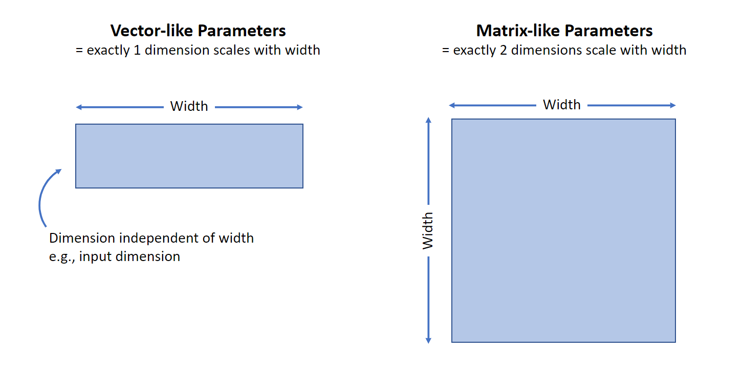 Fig. Vector-like vs Matrix-like. Source from Greg Yang’s Blog
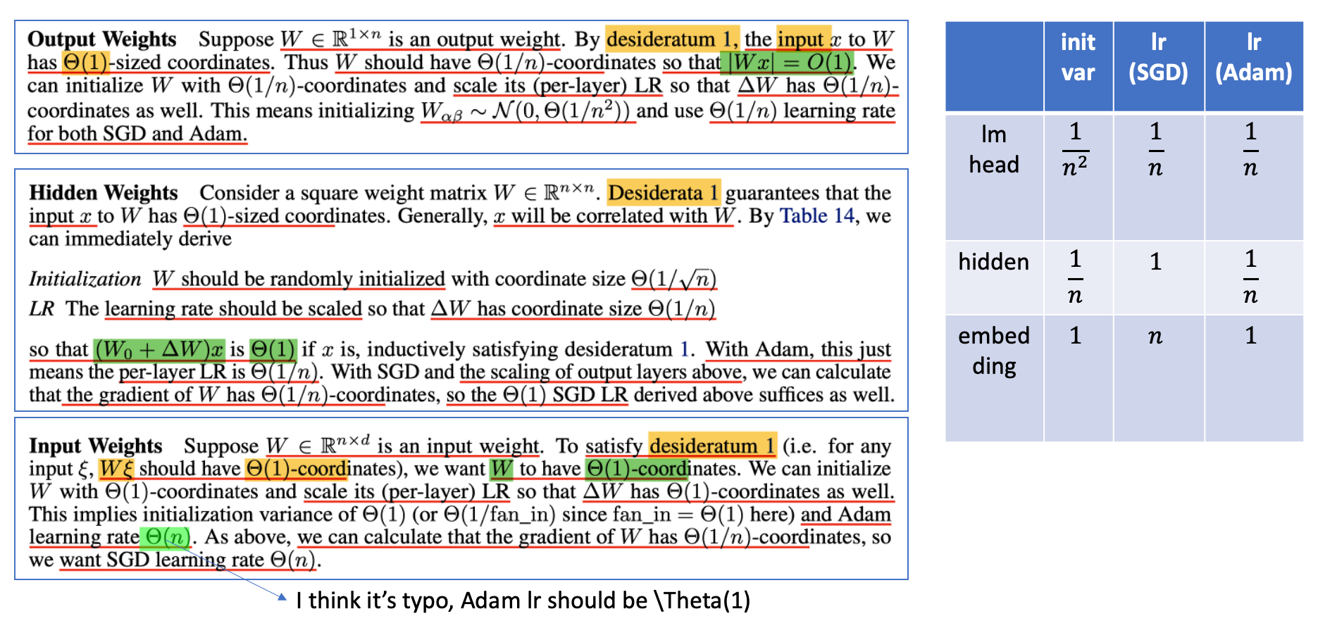
For example, in transformer, embedding and unembedding (lm head or readout) matrix has \(W_{emb} \in \mathbb{R}^{V \times n}\) dimension, where \(V\) is vocab size. and there is only one infinite dimension. So it behaves different and this is why we have to apply separate rule and this is the reason why muP implementation table has 3 category (hidden, embedding, unembedding).
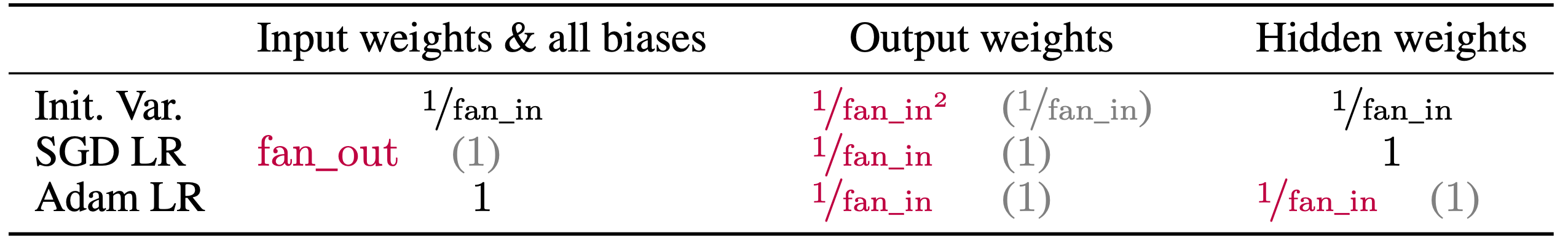 Fig. Openreview of TP-V. Greg Yang explain ‘muP is not only for HP transfer’
Again, to achieve both ‘training stability’, ‘maximal feature learning’, and ‘non-triviality’, we should keep below two things in below three desideratum.
Fig.
Then, we can derive scaling rule for embedding and unembedding matrices, and bias term in similar way.
- Some notes for derivation
- input vector’s coordinate is typically i.i.d and \(\Theta(1)\) because it’s our desideratum (and i guess it’s reasonable because we use input layernorm for every module)
- here \(O(1)\) and \(\Theta(1)\) are different (\(\Theta(1)\) include lower bound), and network output logit, \(y=W_{out}x\) should be \(O(1)\), not \(\Theta(1)\) coordinate
- For the desideratum 2 (network output logit should be \(O(1)\)), it can go to zero at initialization. but the network output should be \Theta(1) after training.
- output weight also perform dot product between n-dim vectors, but it’s variance is different from hidden matrix (\(\sigma^2_{out}=1/n^2\) vs \(\sigma^2_{hidden}=1/n\)) because it should ensure \(\vert Wx \vert = \vert \sum_i W_{out,i} x_i \vert = O(1)\).
- logit gradient \(dL/dy\) is \(\Theta(1)\) (easy to derive using Mean Square Error (MSE) or Cross-Entropy (CE) Loss. it’s not depend on width, \(n\))
- intuitively, to maximize feature learning, it’s acceptable to maintain init weight’s quantity and update quantity in same scale (\(\Delta W / W_{init} \approx \Theta(1)\))
- for hidden matrix, it’s upstream gradient has \(\Theta(1/n)\) coordinate (\(dL/dz \approx \Theta(1/n)\) because \(dL/dz=W_{out} \otimes dL/dy\) and \(W_{out}\) has \(1/n\) coordinate (\(1/n^2\) variance)
- that’s why we can use \(\Theta(1)\) scale lr for hidden matrix when using SGD optimizer
- for embedding matrix in LM, we use one-hot vector and look up embedding, so it does not depend on width, \(n\)
Actually, What muP want to say is simply as follows
- readout (lmhead) layer gets too much gradient, so discount it.
- you should discount lr by \(1/n\) (to counter dot product blow up) as \(n\) grows.
- embedding gets too small gradient, so boost it.
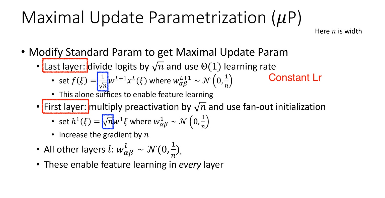 Fig.
Fig.
abc-parameterization
Actually, TP authors defines abc-parameterization for muP, where a stands for multiplier, b for init std, and c for lr per parameters, and we should define this a, b, c to make model behavior does not change when width, n goes to infinity.
-
a: we parameterize each weight parameters as \(W^{l} = n^{-a_l} w^l\) for actual trainable param \(w^l\) -
b: we init each \(w^l \sim \mathcal{N}(0, n^{-2b_l})\) -
c: the SGD lr is \(\eta n^{-c}\) for some width-independent \(\eta\)
(here multipler doesn’t exist in conventional initialization method like Lecun init. it is scaling factor applied after linear transform)
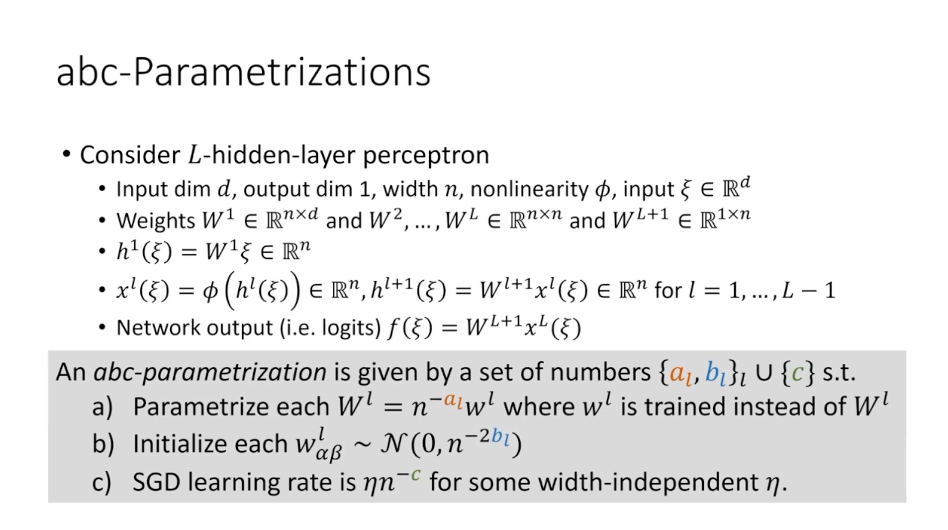
(For simplicity, i didn’t mentioned abc-parameterization earlier but it’s crucial to further understand muP)
And the main Question: “How to correctly we set per layers a, b, c to make every layer’s activation not blown up (training stability) and to be trained equally? (maximal feature learning) as Neural Network (NN)’s width goes to infinity?”
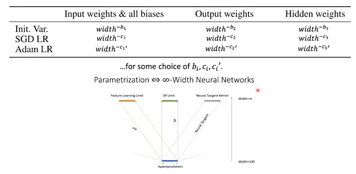 Fig.
Fig.
And the mathematically derived answer to this question is TP 4 and 5, and it ensure maximal feature learning and training stability in inifinite width regime. (like we simply derive above. see papers for more strict and beautiful mathemetical derivation)
Fig. Maximal Update Parameterization Table
And because muP is well defined for any NN building block, it is also valid for Noam architecture where the model consists of Rotary Positional Embedding (RoPE), RMSNorm, and Gated Linear Unit (GLU).
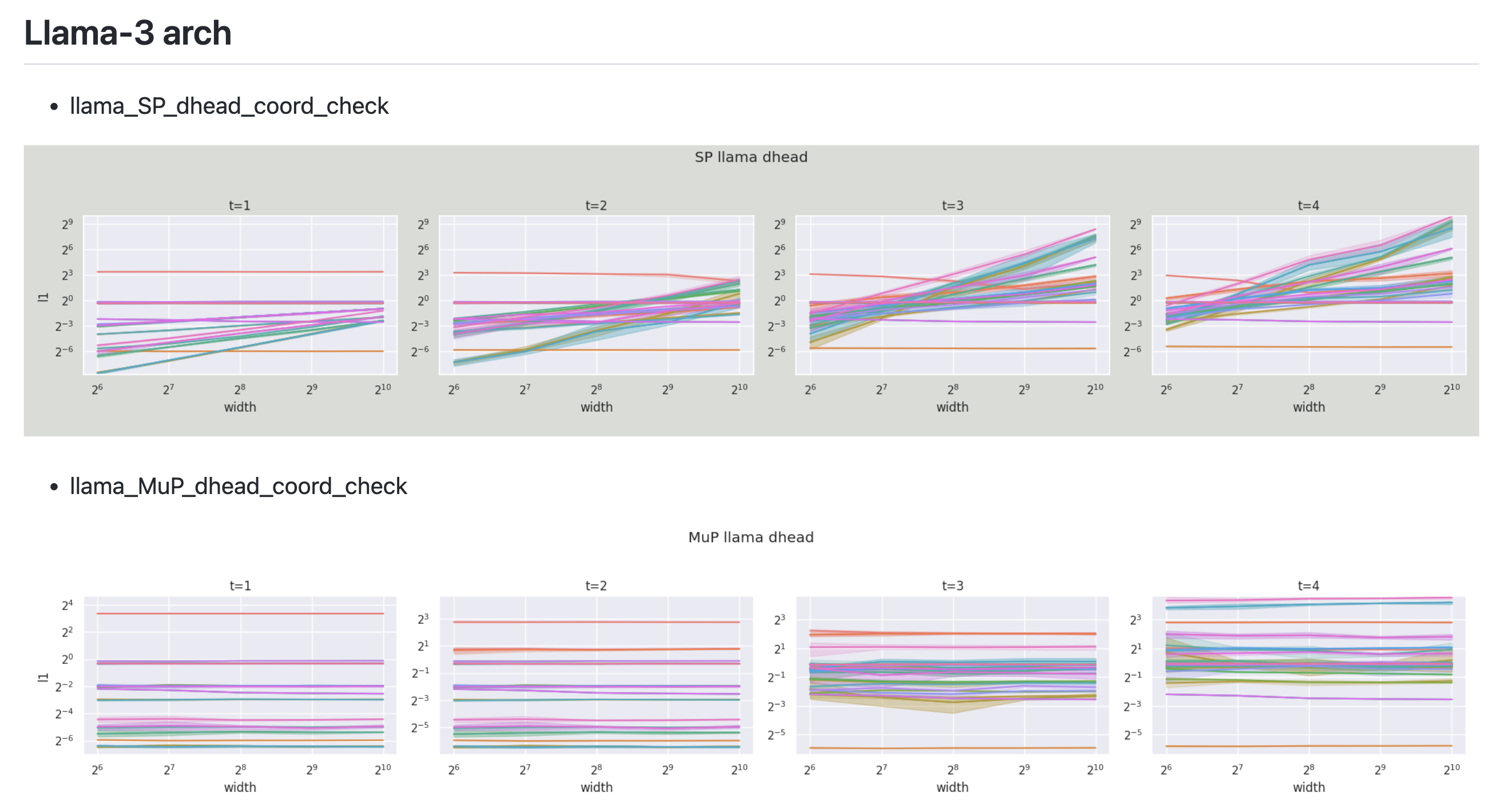 Fig. my coordinate check on LLaMa-3 architecture.
Now, to further understanding and implementing muP with flexiblilty, we’re gonna discuss abc-parameterization symmetry. abc-parameterization symmetry means, if you properly set this a,b,c (multiplier, std, base lr each), NN’s fwd, bwd will stay same. So, this is the reason why there are 3 different (but same) tables in TP-V.
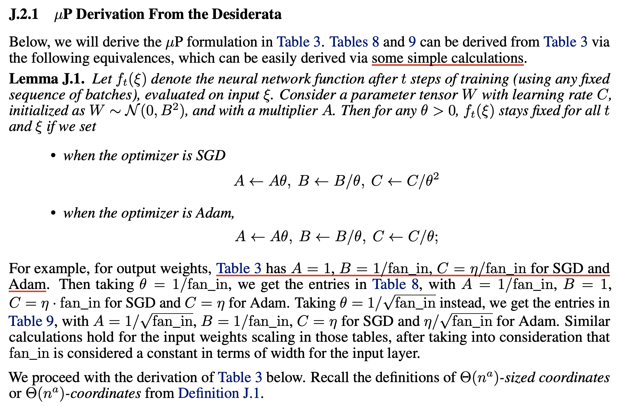 Fig.
Fig.
But 'why do we need alternative forms to implement muP?' This is because one might want to use tie embedding strategy for saving memory or better performance.
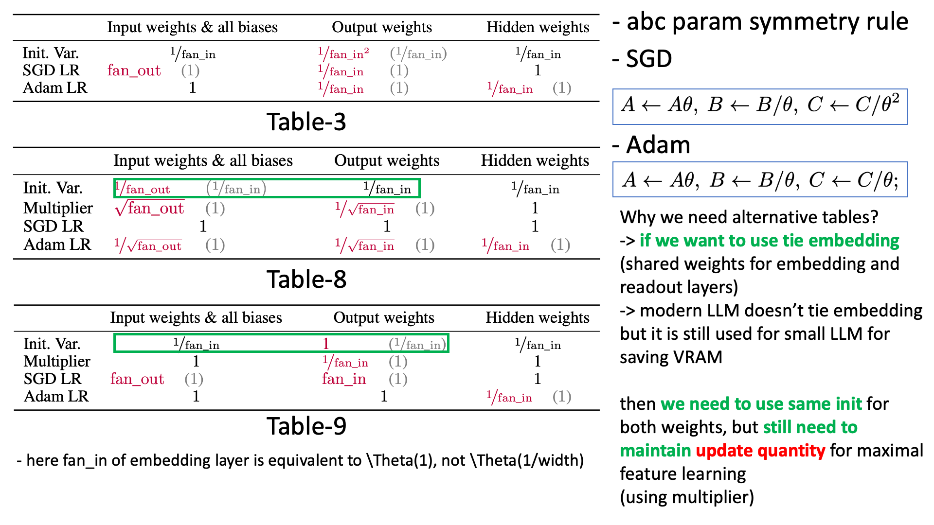 Fig.
Fig.
Simply put, you can accept this rule like “Oh, if the multiplier is scaled by a factor of \(\theta\), then the init std should also be reduced by \(\theta\). And since the model’s init std becomes smaller, the magnitude of its updates should also be scaled down accordingly!”.
Let’s think bout l-th layer’s weight parameter, \(W\).
\[\begin{aligned} & W^l = A W^l & \\ & W^l \sim \mathcal{N}(0, B) & \\ & \eta_{eff} = \eta C & \\ \end{aligned}\]It is easy to prove that l-th layer’s output (pre-activation) stays same in forward if we scale multiplier by \(\theta\) and init std by \(1/\theta\).
\[\begin{aligned} & A \leftarrow A\theta, B \leftarrow B/\theta, C \leftarrow C/\theta^2 & \\ & z_t^l = A \cdot W_t^l x, W_t^l \sim \mathcal{N}(0,B^2) & \\ & = (A \color{red}{\theta}) \cdot \frac{W_t}{\color{red}{\theta}} x & \\ \end{aligned}\]And for backward, if we update weight parameter using SGD (no momentum), it is also easy to implement.
\[\begin{aligned} & z_0^l = A \cdot W_0^l x, W_0^l \sim \mathcal{N}(0,B^2) & \\ & W_{1}^l = W_0^l - \underbrace{C \cdot \eta \cdot(\nabla_{W_0^l}L)}_{\text{SGD Update}} & \\ & = W_0^l - C \cdot \eta \cdot (A \frac{dL}{dz^l_0} x^T) & \\ & z_{1}^l = A \cdot W_{1}^l x' & \\ & = A \cdot (W_0^l - C \cdot \eta (A \frac{dL}{dz^l_0} x^T)) x' & \\ \end{aligned}\] \[\begin{aligned} & A^{\ast}=A\theta, B^{\ast}=B/\theta, C^{\ast}=C/\theta^2 & \\ & {z'}_0^l = A' \cdot W_0^{l\ast} x, W_0^{l\ast} \sim \mathcal{N}(0, {B'}^2) & \\ & = (A \color{red}{\theta}) \cdot \frac{W_0^l}{\color{red}{\theta}} x & \\ & = A \cdot W_0^l x & \\ & z_{1}^{l\ast} = A' \cdot W_{1}^{l\ast} x' & \\ & = A' \cdot (W_{0}^{l\ast} + C' \cdot \eta \cdot \nabla_{W_{0}^{l\ast}}L ) x' & \\ & = (A \color{red}{\theta}) \cdot ( \frac{W_0^l}{\color{red}{\theta}} - \frac{C}{\color{red}{\theta^2}} \cdot \eta \cdot ((A \theta ) \frac{dL}{dz^{l\ast}_0} x^T)) x' & \\ & = z_1^l & \\ \end{aligned}\]For Adam(W) optimizer, there is a difference that lr is scaled by \(1/\theta\), not \(1/\theta^2\). You can easily derive this too because adaptive optimizer already do ‘per parameter lr scaling’.
\[\begin{aligned} & A \leftarrow A\theta, B \leftarrow B/\theta, C \leftarrow C/\theta & \\ \end{aligned}\]Adam update is as follows (adam is scale invariant). (you can check Tensor Programs IVb: Adaptive Optimization in the Infinite-Width Limit to further understanding.)
\[\begin{aligned} & z_0^l = A \cdot W_0^l x, W_0^l \sim \mathcal{N}(0,B^2) & \\ & G_0 = \nabla_{W_0^l} L = A \frac{dL}{dz_0^l} x^T & \\ & m_0 = \beta_1 m_{init} + (1-\beta_1) G_0 & \\ & v_0 = \beta_2 v_{init} + (1-\beta_2) (G_0)^2 & \\ & \hat{m_0} = m_0/(1-b_1^0) & \\ & \hat{v_0} = v_0/(1-b_2^0) & \\ & \Delta {W_0^l} = \underbrace{\frac{\hat{m_0}}{\sqrt{\hat{v_0} + \epsilon}}}_{\text{Adam Update}} & \\ & z_{1}^l = A \cdot W_{1}^l x' & \\ & = A \cdot (W_0^l - C \cdot \eta \Delta {W_0^l}) x' & \\ \end{aligned}\] \[\begin{aligned} & A^{\ast}=A\theta, B^{\ast}=B/\theta, C^{\ast}=C/\theta & \\ & {z}_0^{l\ast} = A' \cdot {W}_0^{l\ast} x, {W}_0^{l\ast} \sim \mathcal{N}(0,{B'}^2) & \\ & = (A \color{red}{\theta}) \cdot \frac{W_0^l}{\color{red}{\theta}} x & \\ & = A \cdot W_0^l x & \\ & G'_0 = \nabla_{W_0^{l'}} L = (A\color{red}{\theta}) \frac{dL}{dz_0^l} x^T & \\ & \Delta W_0^{l\ast} = \frac{\hat{m^{\ast}_0}}{\sqrt{\hat{v^{\ast}_0} + \epsilon}} = \frac{\theta \hat{m_0}}{\sqrt{\theta^2 \hat{v_0} + \epsilon}} & \\ & \approx \nabla_{W_0^l}L & \\ & z_1^{l\ast} = (A \color{red}{\theta}) \cdot (\frac{W_0^l}{\color{red}{\theta}} - \frac{C}{\color{red}{\theta}} \cdot \eta \Delta W_0^{l\ast}) x' & \\ & = z_1^l & \\ \end{aligned}\]# https://arxiv.org/abs/2310.02244
# https://x.com/thecharlieblake/status/1799029085827649930
import torch
from torch import manual_seed, nn, optim, randn
def get_second_fwd_output(mult, init_std, lr, opt):
assert opt in [optim.Adam, optim.SGD]
manual_seed(1234)
l = nn.Linear(1024, 2048, bias=False)
nn.init.normal_(l.weight, std=init_std)
model = lambda x: l(x) * mult
args = {'lr':lr, 'eps':0} if opt==optim.Adam else {'lr':lr}
opt = opt(l.parameters(), **args)
x = randn(512, 1024).requires_grad_()
y1 = model(x).mean()
y1.backward(); opt.step()
y2 = model(x).mean()
print(y1, y2)
return y2
def adjust_sgd(mult, init_std, lr, theta):
return mult*theta, init_std*theta**-1, lr*theta**-2
def adjust_adam(mult, init_std, lr, theta):
return mult*theta, init_std*theta**-1, lr*theta**-1
theta = 2.5
mult = 1; init_std = 0.02; lr = 1
assert torch.allclose(
get_second_fwd_output(mult, init_std, lr, opt=optim.Adam),
get_second_fwd_output(*adjust_adam(mult, init_std, lr, theta), opt=optim.Adam),
)
assert torch.allclose(
get_second_fwd_output(mult, init_std, lr, opt=optim.SGD),
get_second_fwd_output(*adjust_sgd(mult, init_std, lr, theta), opt=optim.SGD),
)
tensor(2.5274e-05, grad_fn=<MeanBackward0>) tensor(-35.6423, grad_fn=<MeanBackward0>)
tensor(2.5274e-05, grad_fn=<MeanBackward0>) tensor(-35.6423, grad_fn=<MeanBackward0>)
tensor(2.5274e-05, grad_fn=<MeanBackward0>) tensor(-0.0009, grad_fn=<MeanBackward0>)
tensor(2.5274e-05, grad_fn=<MeanBackward0>) tensor(-0.0009, grad_fn=<MeanBackward0>)
muP is not Silver Bullet (across the batch size and training horizon)
Now we know how to scale up model size , we know how to transfer optimal HPs from small-scale proxy experiments.
However, even though muP is theoretically well-defined,
it does not guarantee HP transfer across training tokens or batch size.
Especially, the fact that ‘muP does not ensure HP transfer across training horizon’ is not widely spread.
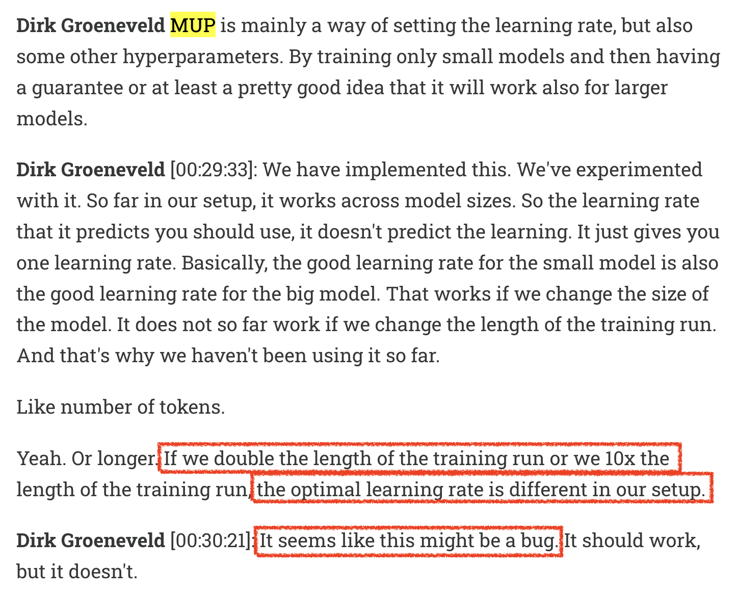 Fig. It may be not a bug. Source from Interview on OLMo team
Let’s consider increasing the training horizon.
For example, suppose we train a small-scale proxy model (40M parameters) with 10B tokens,
and we want to transfer the optimal lr to a 70B model trained on 10T tokens.
Will the optimal lr remain the same? maybe, not.
Intuitively, the model will remain at its peak lr longer if training horizon is scaled up.
So we should counter this, we should decrease lr if we want to transfer lr. This leads to a left-shift trend in the optimal lr curve even though you use muP
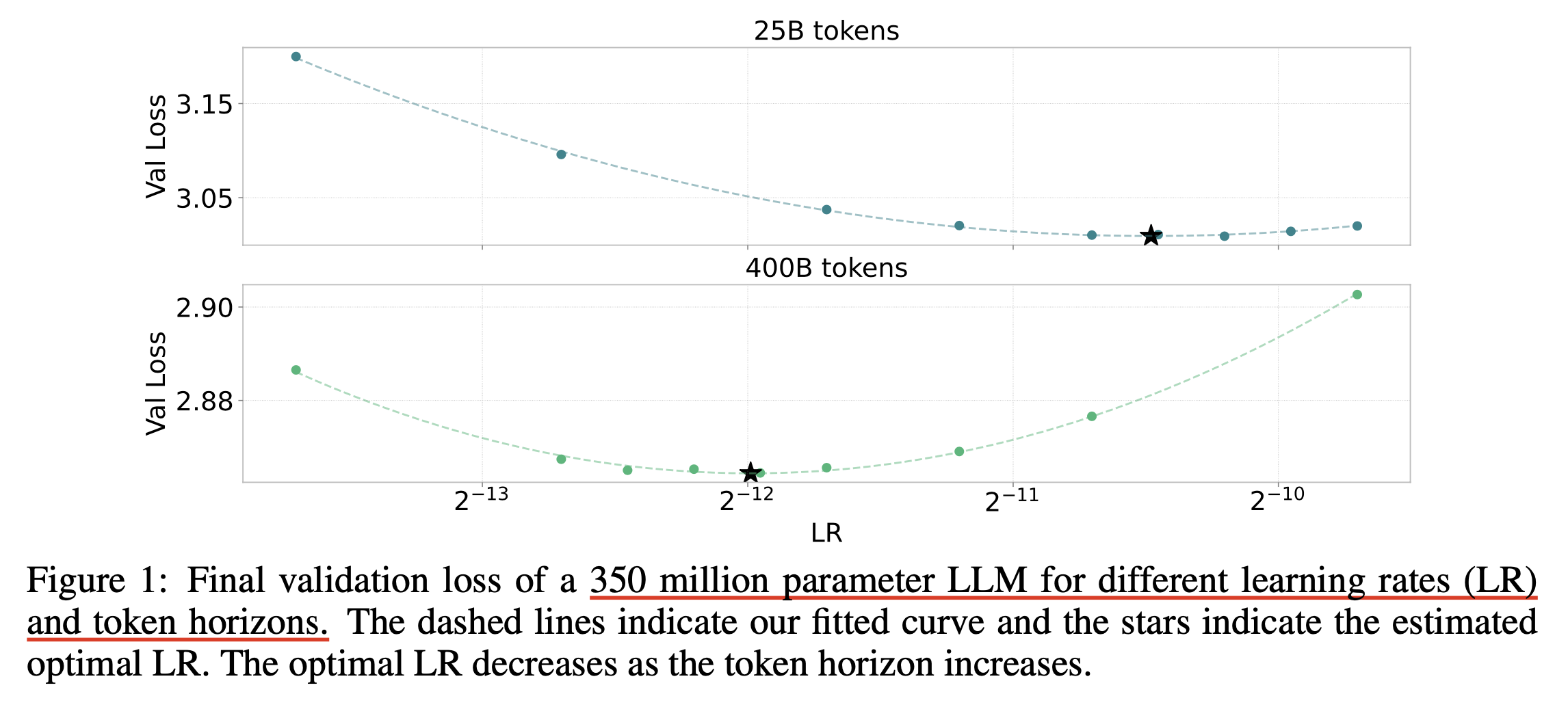 Fig. left shift trends. Source from Scaling Optimal LR Across Token Horizons
Now consider bsz.
It’s common to increase the bsz when training larger models to achieve better training efficiency (throughput).
(As long as you don’t cross the critical bsz , we’ll discuss that later.)
But increasing bsz reduces training steps.
So we can think like
“Hmm, gradients are more accurate but training steps are fewer, so let’s raise the lr to compensate.”
In other words, to counter the shortened training horizon,
we must increase lr, and this leads to a right-shift trend to reach the same validation loss as smaller batch training. And conventional rule for bsz-lr scaling rule is sqrt(n). (you can see this post from Sadhika Malladi for more)
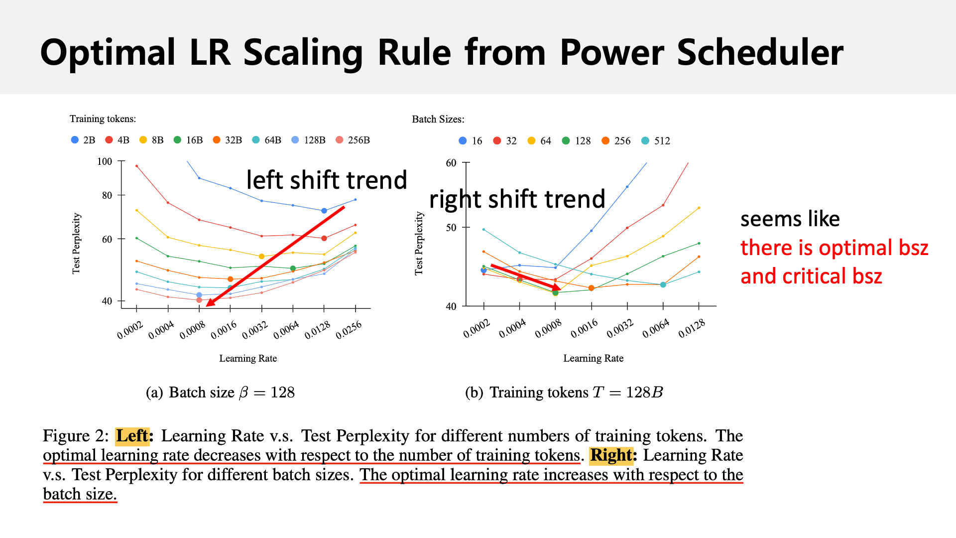 Fig. Soruce from Power Scheduler: A Batch Size and Token Number Agnostic Learning Rate Scheduler
In the TP-V paper, the authors show that lr can be transferred well across bsz,
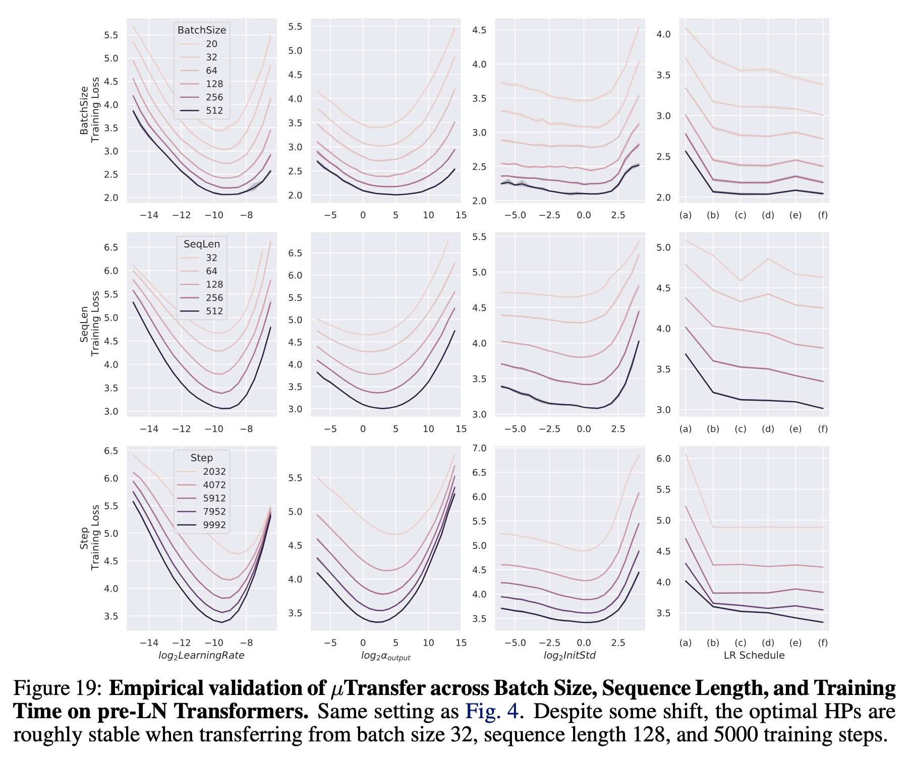 Fig.
Fig.
but you should not overlook they use “same training steps” for this experiment. That means they used more FLOPs for increased bsz setup and they don’t need to care bout bsz-training step tradeoff.
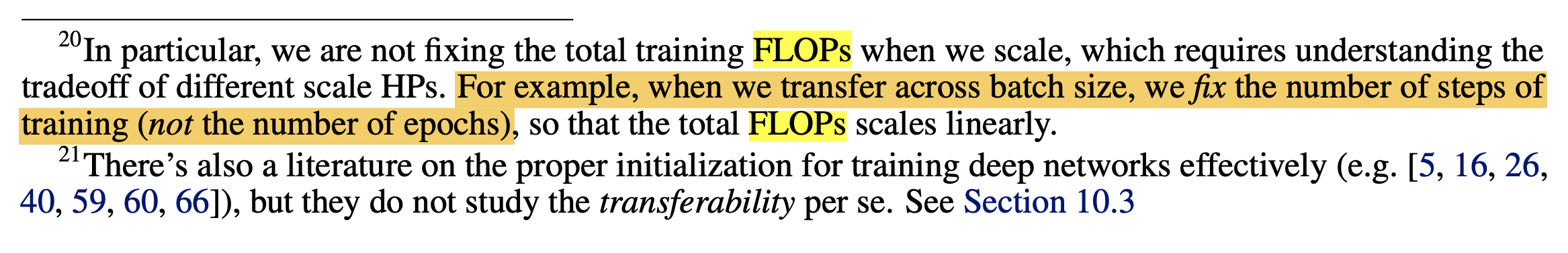 Fig. Source from TP-V
So, if we want to scale both model size and training horizon (tokens, bsz),
we need to understand optimal lr scaling for all three dimensions. muP doesn’t tell us how to adjust lr with respect to bsz or training tokens.
Outdated) Overall Scaling Rule using muP
- Updated) note that, this scaling table is outdated now (Dec 31st 2025), currently many researchers have been exploring scaling rule for weight decay, adam(w) hparams like epsilon, beta 1, 2. Completed Hyperparameter Transfer across Modules, Width, Depth, Batch and Duration propose the ultimate scaling table across width, depth, batch size and training horizon. so, i recommend to read this paper.
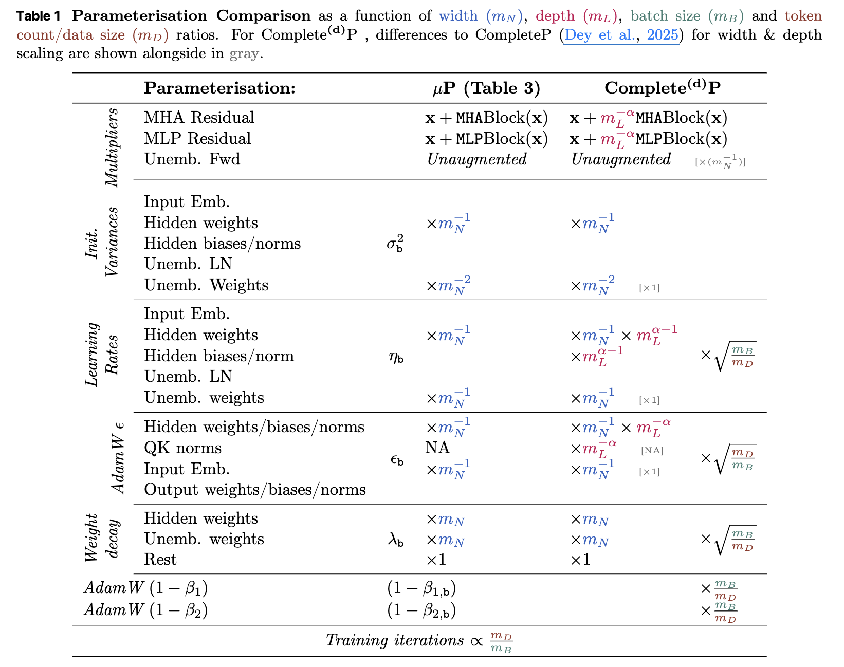 Fig.
Fig.
But i leave this subsection for your information.
This table is primarily derived from Tensor Program (TP) 4 and 5.
It assumes that model size growth is based only on width (hidden size or embedding size), not depth (number of layers), and that you’re using an adaptive optimizer like Adam. Also, as discussed earlier, some scaling rules (like LR vs. bsz and training horizon) are based on my interpretation and findings from several papers. This table is heavily inspired by ‘What to do to scale up?’ from Simo Ryu.
Note that this table is not optimal. it is only an example guideline for motivation. Some parts may be incorrect, so you should determine each component’s scaling factor, since optimization hyperparameters (such as beta 1, 2, weight decay, lr, and bsz) are intricately correlated and few of them are discovered afaik. you still theoretically or empirically find their correlation.
| hparams | embedding | hidden | residual_out | unembedding (readout) |
|---|---|---|---|---|
| init_std (b) | \(\sigma_\text{embed}\) | \(\sigma_\text{hidden} \cdot (\color{red}{\tilde{n}})^{-0.5}\) | \(\sigma_\text{res-out} \cdot (\color{red}{\tilde{n}})^{-0.5} \cdot (2 n_\text{layers})^{-0.5}\) | \(\sigma_\text{un-embed}\) |
| multiplier (a) | \(\alpha_{\text{embed}} \cdot 1\) | \(\alpha_{\text{hidden}} \cdot 1\) | \(\alpha_{\text{res-out}} \cdot 1\) | \(\alpha_{\text{un-embed}} \cdot (\color{red}{\tilde{n}})^{-1}\) |
| adamw lr (c) | \(\eta_{\text{embed}} \cdot (\color{green}{\tilde{b}})^{0.5} \cdot {(\color{blue}{\tilde{d}})^{\alpha_{\text{data}}}}\) | \(\eta_{\text{hidden}} \cdot (\color{red}{\tilde{n}})^{-1} \cdot (\color{green}{\tilde{b}})^{0.5} \cdot {(\color{blue}{\tilde{d}})^{\alpha_{\text{data}}}}\) | \(\eta_{\text{res-out}} \cdot (\color{red}{\tilde{n}})^{-1} \cdot (\color{green}{\tilde{b}})^{0.5} {(\color{blue}{\tilde{d}})^{\alpha_{\text{data}}}}\) | \(\eta_{\text{un-embed}} \cdot (\color{green}{\tilde{b}})^{0.5} {(\color{blue}{\tilde{d}})^{\alpha_{\text{data}}}}\) |
| adamw moment | \((1-\color{green}{\tilde{b}}(1-\beta_1),\\1-\color{green}{\tilde{b}}(1-\beta_2))\) | \((1-\color{green}{\tilde{b}}(1-\beta_1),\\1-\color{green}{\tilde{b}}(1-\beta_2))\) | \((1-\color{green}{\tilde{b}}(1-\beta_1),\\1-\color{green}{\tilde{b}}(1-\beta_2))\) | \((1-\color{green}{\tilde{b}}(1-\beta_1),\\1-\color{green}{\tilde{b}}(1-\beta_2))\) |
| adamw epsilon | \(\epsilon \cdot (\color{green}{\tilde{b}})^{-0.5}\) | \(\epsilon \cdot (\color{green}{\tilde{b}})^{-0.5}\) | \(\epsilon \cdot (\color{green}{\tilde{b}})^{-0.5}\) | \(\epsilon \cdot (\color{green}{\tilde{b}})^{-0.5}\) |
| adamw weight_decay | \(\lambda \cdot (\tilde{b}^?) \cdot (\tilde{d}^?)\) | \(\lambda \cdot (\tilde{n}) \cdot (\tilde{b}^?) \cdot (\tilde{d}^?)\) | \(\lambda \cdot (\tilde{n}) \cdot (\tilde{b}^?) \cdot (\tilde{d}^?)\) | \(\lambda \cdot (\tilde{b}^?) \cdot (\tilde{d}^?)\) |
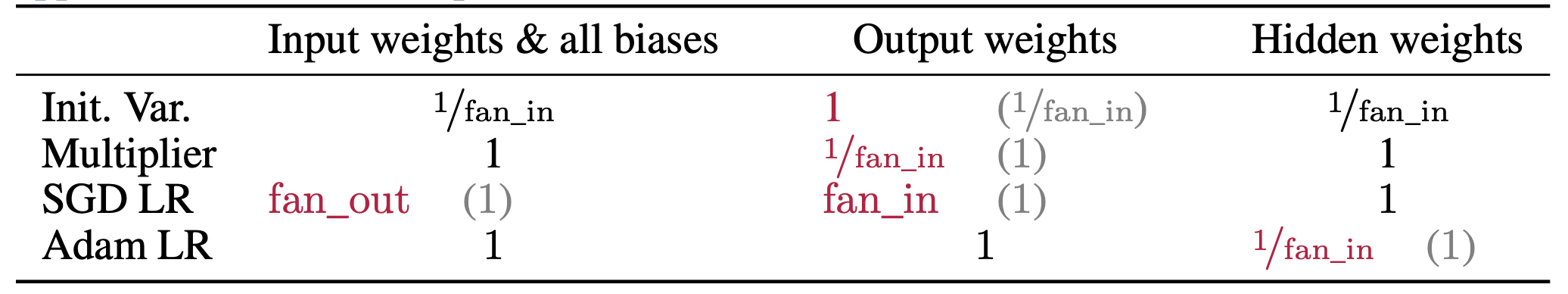 Fig. Table 8 from TP-V
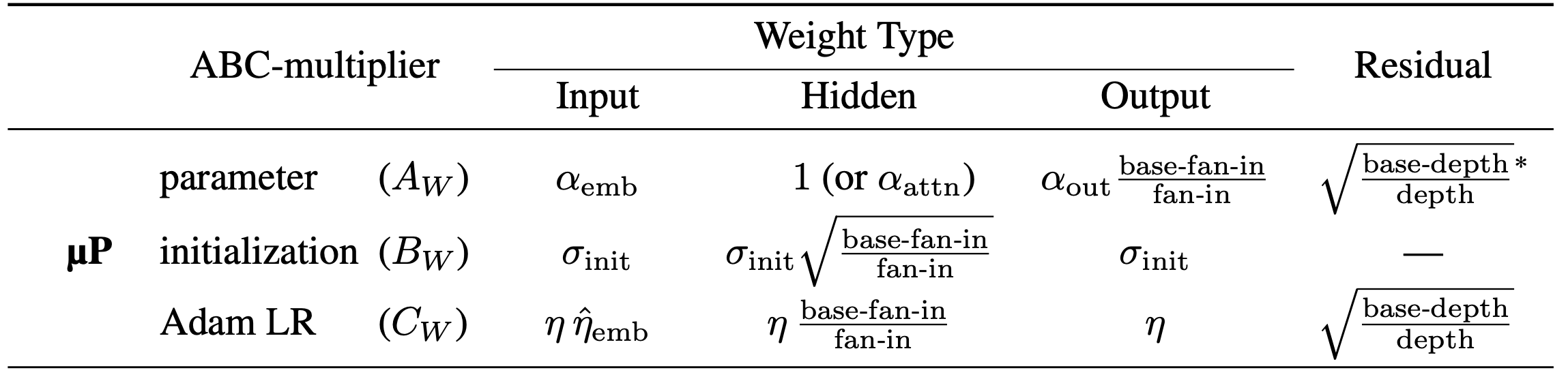 Fig. Table 2 from unit-muP. it is based on Table 8 from TP-V but also reflects depth scaling from TP-VI (see residual branch’s multiplier)
-
width: Width refers to the hidden size (or head dimension) of a neural network (e.g., in Transformers). For small-scale proxy (base) models, the shape of a specific layer’s weight matrix is given by \(W_l \in \mathbb{R}^{\text{fan-in}_\text{base} \times \text{fan-in}_\text{base}}\). In TP-5, Tables 3, 8, and 9 describe parameterization in terms offan_inandfan_out, corresponding to input and output feature dimensions. In this table, we define \(\tilde{n} = \text{fan-in} \cdot \frac{1}{\text{fan-in}_\text{base}}\). If \(\text{fan-in}_\text{base} = 1\), it recovers to Table 8. For example, if \(\sigma = 1/\sqrt{1024} \approx 0.031\), then init std becomes \(1/\text{fan-in}\).- e.g.: \(\color{red}{\tilde{n} = 100}\)
-
multiplier- Note that there are two multipliers: one for width scaling and one for HPs.
For example, embedding outputs may be defined asx = hparam_multiplier × width_scaling_multiplier × embedding_layer(x),
wherewidth_scaling_multiplierremains constant as width increases, andhparam_multiplierrefers to things like lr. - A common choice is \(\alpha_{\text{embed}} = 10\) (based on various muP-related studies), with width scaling multiplier set to 1.
- Although this table uses a shared \(\sigma\) and lr across all parameters, you can specify per-layer values for init std, lr, and multipliers if desired.
- Note that there are two multipliers: one for width scaling and one for HPs.
-
residual branch's output layers- It’s well-known that residual outputs should be scaled by \(\frac{1}{\sqrt{2L}}\) where \(L\) is the number of layers (depth). This is because residual blocks add the original input twice per block, resulting in \(2L\) additions. This scaling is compatible with muP and is discussed in TP-6.
-
attention logit scaling- Scaled Dot-Product Attention (SDPA) is also a dot product. In muP, the scaling should be \(d_\text{head}\) instead of \(\sqrt{d_\text{head}}\) in the \(QK^T / \text{scale}\) term. This is because \(q\) and \(k\) become correlated after training begins, so scaling should follow the Law of Large Numbers (LLN). Attention operators may have an
attn_multiplier, but we typically set it to 1.0.- Notably, the original Attention is All You Need paper uses \(\sqrt{d_\text{head}}\) because \(q\) and \(k\) are i.i.d. at initialization, this is SP behavior, not muP (LLN vs. CLT).
- Scaled Dot-Product Attention (SDPA) is also a dot product. In muP, the scaling should be \(d_\text{head}\) instead of \(\sqrt{d_\text{head}}\) in the \(QK^T / \text{scale}\) term. This is because \(q\) and \(k\) become correlated after training begins, so scaling should follow the Law of Large Numbers (LLN). Attention operators may have an
 Fig. I also overlooked this note from Attention Is All You Need paper. they designed transformer modules in literally every point of views (stability, parallelizability, …).
- LR scaling
across bsz- If we increase bsz by \(n\), the number of training steps decreases, so lr should be scaled by \(\sqrt{n}\).
We define:
\(\tilde{b} = \text{bsz} / \text{bsz}_\text{base}\) - e.g. \(\color{green}{\tilde{b} = 8}\) (e.g., 4M for target model and 500K for small-scale proxy)
- lr scaling should be \(\eta \cdot \tilde{b}^{0.5}\). (Not necessarily optimal, but a well-known heuristic.)
- Note that, we should care bout Critical Batch Size (cbsz). If bsz exceeds this threshold, training efficiency no longer improves. (we will discuss later). So, don’t just use the largest bsz your GPUs allow. Choose one that maintains high Machine FLOPs Utilization (MFU).
- If we increase bsz by \(n\), the number of training steps decreases, so lr should be scaled by \(\sqrt{n}\).
- LR scaling
across dataset size- This is less theoretically grounded as far as i know.
- Typically, small-scale proxies use far fewer tokens (e.g., 1/100 of the target tokens).
- Define: \(\tilde{d} = \frac{d_\text{large}}{d_\text{small}}, \quad \alpha_\text{data} = \text{scaling exponent}\)
- e.g. If \(d_\text{large} = 8T\) and \(d_\text{small} = 80B\), then \(\tilde{d} = 100\).
- There’s no known theoretical formula for \(\alpha_\text{data}\), but Scaling Exponents Across Parameterizations and Optimizers suggests \(-0.12\) for Chinchilla-style scaling. Given \(N \sim n^2\), the rule becomes \(n^{-1} \cdot n^{2 \cdot -0.12} = n^{-1.24}\) (authors never claim this value is right scaling rule. it’s just simply derived following chinchilla).
 Fig. contribution of increased dataset size in compute optimal setup
-
What HPs should we tune?- There are many to tune: \(\eta_{\text{embed}}, \eta_{\text{hidden}}, \sigma_{\text{embed}},\) etc.
- In practice, most use the same global lr and init std for simplicity even though it’s probably suboptimal.
-
Zero-variance initialization:
It’s recommended to use zero initialization to eliminate discrepancies between small and large models (see TP-V and NNGP).- Query projection matrix
- Residual output (residual branch’s output layers e.g., out projection, FFN FC2 projection)
- LM head (readout)
- Other Optimizer HPs:
Use \((\beta_1, \beta_2) = (0.9, 0.95)\) and \(\epsilon = 1\text{e-}8\), standard for large-scale transformers.- If scaling bsz with compute budget, some suggest using larger \(\beta\) for smaller batches.
- For Weight Decay (WD), \(\lambda\), you can diable this for small scale proxy, and re-actiavte in target scale.
- but be careful it depends on what framework you use. for
tensorflow adamwortruly decoupled adamwdefualt is 1e-4 because pytorch default multiply WD value by lr.- recently proposed papers related to muP claims truly decoupled adamw fixes HP transfer stability
- it’s easy to implement by setting
weight_decayasweight_decay / group['lr']
- it’s easy to implement by setting
- recently proposed papers related to muP claims truly decoupled adamw fixes HP transfer stability
For WD, it is noteworthy that default pytorch adamw is actually coupled with lr. In my experiments with over 200B tokens and 8B++ model sizes,
I experience that loss spikes and finally diverges.
This is because in large scale NN training, mutransfered model’s effective lr for hidden matrices become very small compared to small scale proxy. And because WD is coupled iwth lr, discounted per-parameter lr for hidden matrices makes WD extremely small, and param norm growth never recovered even lr keep decreased by scheduler.
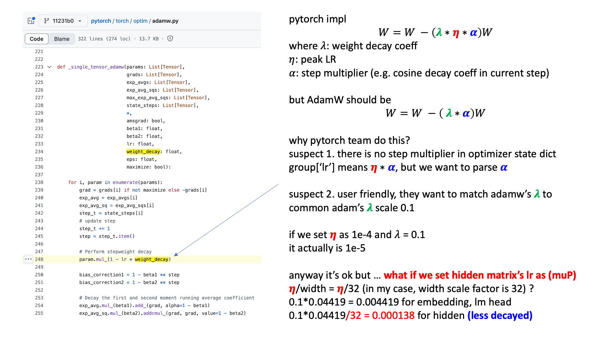
So I strongly recommend using truly independent weight decay, not the PyTorch default.
Why SP can't admit feature learning or HP transfer and is it true?
Although muP is theoretically well-defined and Greg Yang claims it’s a unique solution, it may offer only marginal performance improvements over other parameterizations or muP variants in practice.
In fact, even Standard Parameterization (SP) with a \(1/n\) lr scale can exhibit HP transferability.
 Fig.
Fig.
According to Small-scale proxies for large-scale Transformer training instabilities,
a muP variant called muP (simple) adopts only the \(1/n\) LR scaling from muP while still using fan-in variance,
and yet it successfully transfers optimal lr across width.
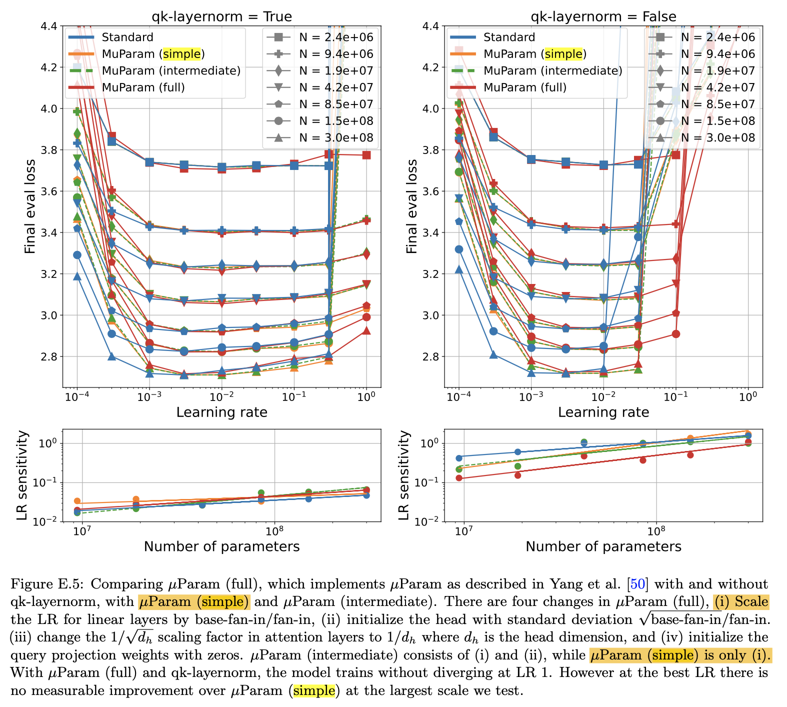 Fig. Small-scale proxies for large-scale Transformer training instabilities
Moreover, GDM shows that every parameterization can admit HP transfer with the right adjustments,
and even reports that SP, with a novel per-layer lr schedule outperforms muP in some cases.
(Though, whether SP + per-layer LR can still be considered “SP” is debatable.)
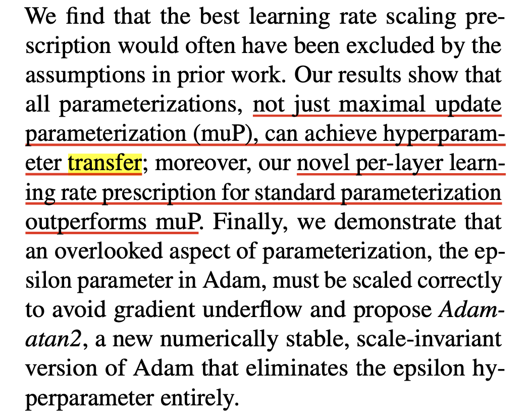 Fig. Scaling Exponents Across Parameterizations and Optimizers
OG Transformer, PaLM and Gemma Parameterization
How did earlier papers approach parameterization?
Surprisingly, papers like Attention Is All You Need and the Pathways Language Model (PaLM) share a few common traits.
First, in the original Transformer paper, it is mentioned that the embedding matrix is multiplied by \(\sqrt{d_{\text{model}}}\).
However, there is no detailed explanation of the initialization method or the reasoning behind this scaling.
The only specific note is that the embedding and language modeling (LM) head weights are tied (i.e., shared).
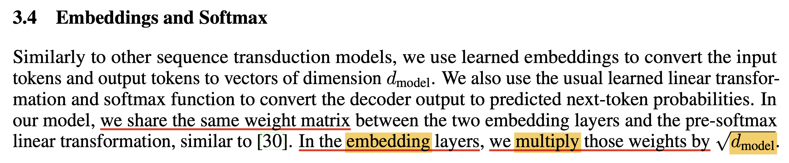 Fig.
Fig.
There are some discussions about this, but it is unclear for me. It’s like “sinusoidal embedding’s scale is bounded by (-1, 1), so embedding matrix should be scaled by sqrt of hidden size”, but i don’t know what init std is.
- Updated) I found a reference from Adafactor paper,
and it turns out the motivation is to ensure that the very first embedding features have unit norm,
while keeping update magnitudes consistent across all matrices.
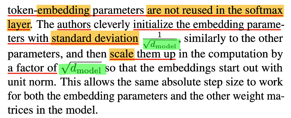 Fig.
Fig.
In PaLM, researchers uses different parameterization. (I call this parameterization, not just initialization, because they adopt Adafactor instead of Adam, allowing per-layer lr, which is quite similar in spirit to muP.) They keep tied embeddings, set init std to 1, and scale the pre-softmax logits by \(1/\sqrt{n}\), where \(n\) is equivalent to \(d_{\text{model}}\).
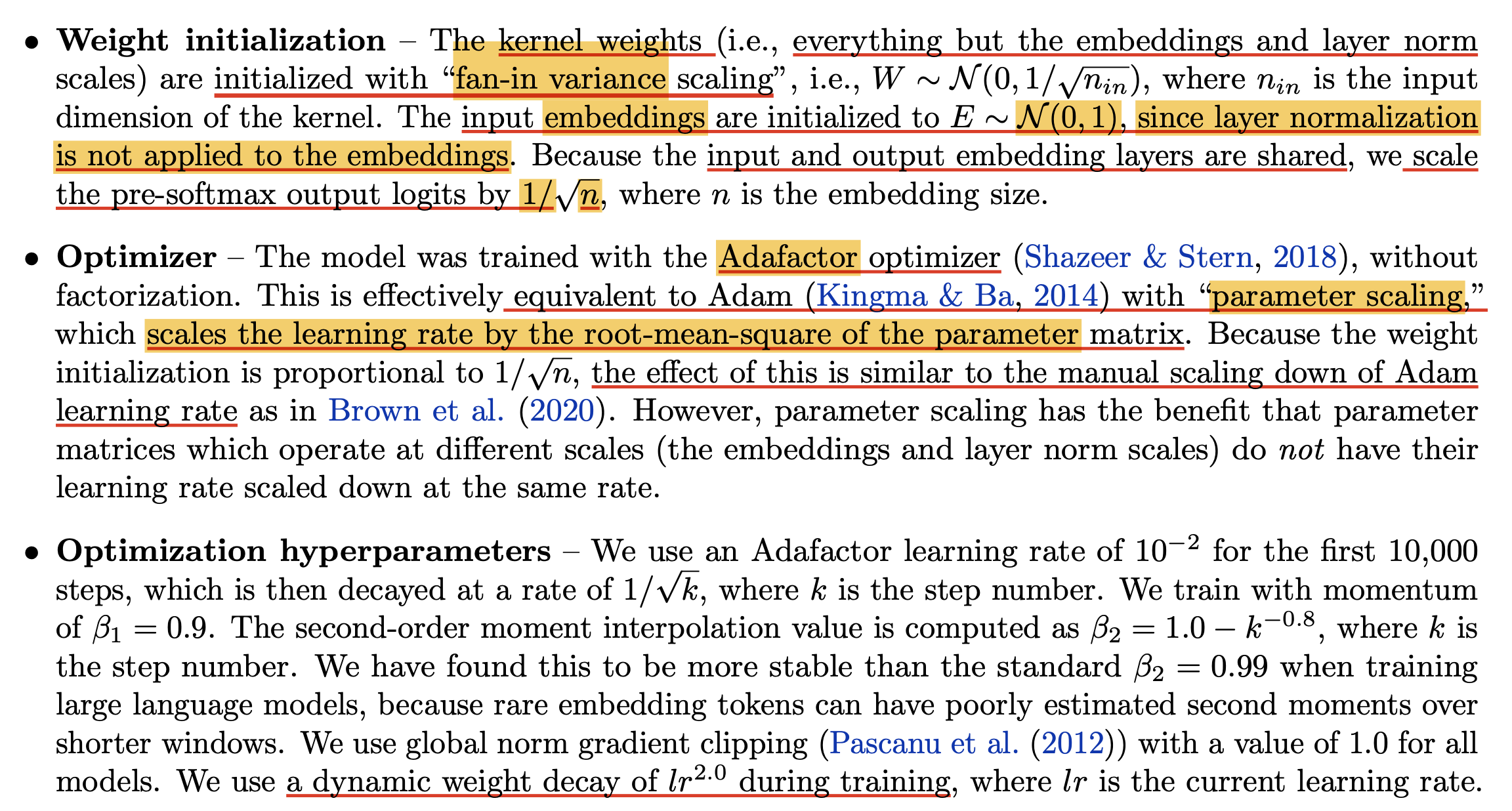 Fig.
Fig.
As the text states, LayerNorm modules normalize their inputs, which means the variance of the outputs is 1.
So it’s reasonable to initialize the embedding matrix with standard deviation 1, this is consistent with muP.
However, the \(1/\sqrt{n}\) logit scaling does not match the \(1/n\) scaling used in muP,
but i believe perhaps Adafactor compensates for this mismatch by adapting the update scale.
Finally, in Gemma-2 and Gemma-3, we can check that GDM continues to try to apply proper parameterization.
 Fig.
Fig.
Some Research Question
Assume you train Mixture of Experts (MoE) model. What init std, and effective lr should we use for sparsely activated Feed Forward Neural Network (FFN)? Indeed, MoE is large FFN but only partial weight matrix is activated dynamically.
Sometimes we treat MoE’s FFN as very big like num_experts X activated FFN size and sometimes as just activated FFN size. It’s kinda complicated because as far as i know when we measure “how we effieicntly train compared to dense”, we use later one, but for fitting HP Scaling Law or measuring cbsz, we use former one. Then what fan-in number should we use?
Also, MoE consumes different the number of tokens compared to attention module. And in MoE training, effective bsz are different for attn and FFN modules because MoE is sparsely activated according to tokens. Assume Global batch size (gbsz) is \(N\), then attn module will consume \(N\) tokens, but FFN consumes \(\frac{N}{E}\times K \times 1.0\) if topk=K, num_exeprts=E, capacity=1.0, Expert Parallelism (EP)=1. So, gradient noise scale from each modules may be different. Then should we scale down lr compared to attn? What per layer lr, init std and bsz should we use for FFNs compared to dense? Does muP can be compatible with MoE? (in my experiments, yes it does but init std of FFN affects performance a lot)
In Switch Transformers, they discount init std, and Efficient Large Scale Language Modeling with Mixtures of Experts reduce lr for FFN for training stability. However, idk it is good solution, especially for reducing lr. in Skywork-MoE, they reduce lr for FFN modules, it seems to work but baseline (not adjust lr for FFN) beats this lr adjusted version in the end.
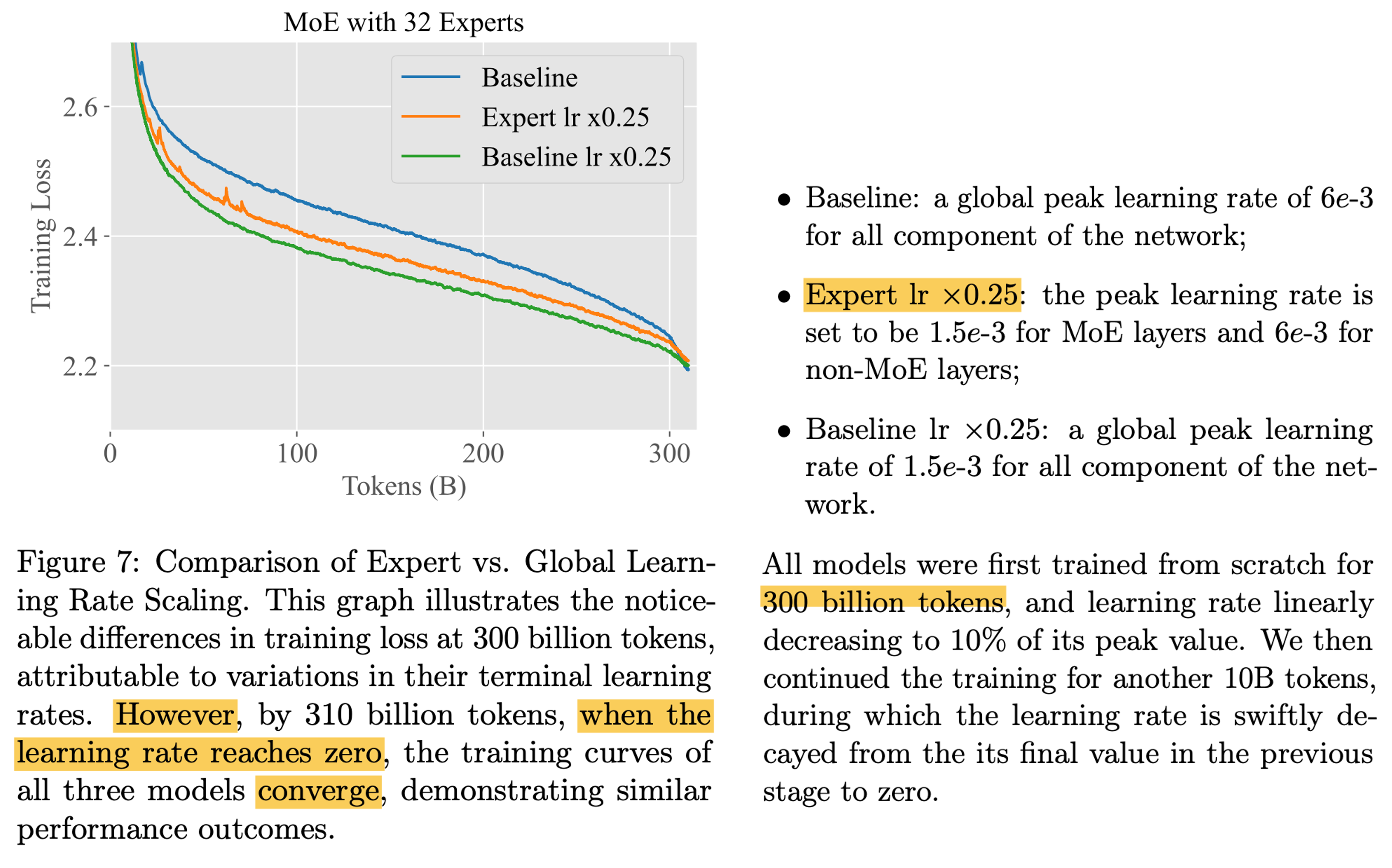
Why? i guess adjusted lr method can cause imbalanced update quantity between ffn’s and attn’s, so it breaks maximal update.
And there is another problem like MoE module’s output (Root Mean Square (RMS) or L2 norm) is relatively small compared to attn module because for backpropagation, typically MoE module output is multiplie by it’s gating score.
\[y = \sum_i^E \underbrace{G_i(x)}_{\text{gating score} \in [0, 1]} \cdot FFN_i(x)\]So, DeepSeek tries to multiply some factor to match output scale with attention module,
 Fig. from DeepSeek-V2
and i guess this value depeneds on how many routed expert we use, and what gating function do we use (sigmoid or softmax).
 Fig.
Fig.
Finally, though it seems to allow HP transfer well across various tasks and model architectures from computer vision and language modeling domain,
 Fig. From my experiments, muP can be applied to almost every architectures including MoE or something because everthing is built on top of dot product and addition
 Fig. muP on various tasks and architectures such as Diffusion Transformer (DiT), Diffusion Language Modeling (LLaDa) and MoE. all credits: cloneofsimo
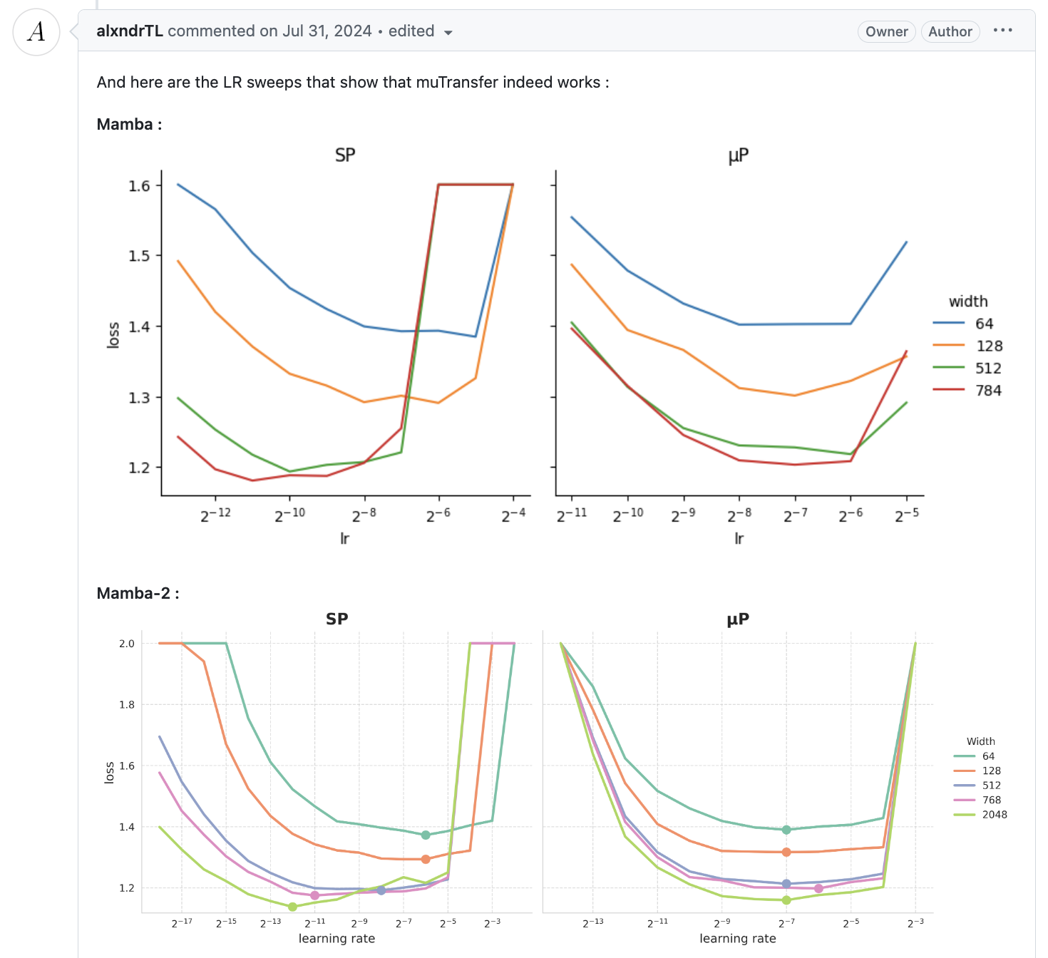 Fig. muP works succesfully on Mamba architectures. Source
I’d like to say there is still many room to do in advanced architectures like MoE (even though MoE for deep neural networks is popularized in 2017 by Noam Shazeer) or something newly proposed models. (from Simo’s work and my experiences, it seems that MoE is compatible with muP but in my experience, MoE is bit sensitive to init std and output scale of routed experts in some large scale)
- Updated) Jingyuan Liu, the 1st author of Muon is Scalable for LLM Training, mentioned it is very important to match Root Mean Squared (RMS) scale of each module’s output (especially routed experts and shared expert) to prevent expert collapse. (see appendix of moonlight paper)
 Fig. Source tweet
 Fig. Source tweet
How to Scale Dataset Size (HP Scaling Law, (Critical) Batch size...)
Updated) Scaling Training Horizion By Adjusting Weight Decay
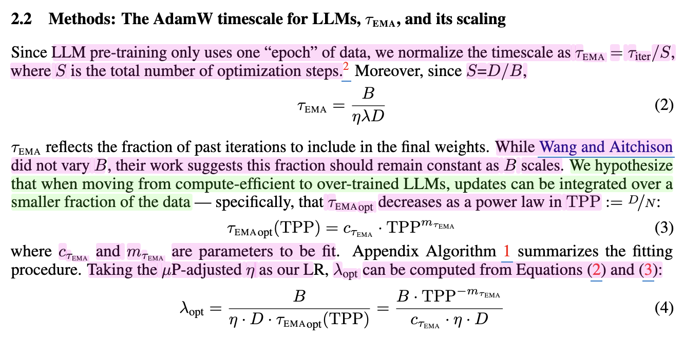
As discussed above, even muP does not guarantee hyperparameter (HP) transfer across training tokens or bsz. However, following Wang et al. (How to set AdamW’s weight decay as you scale model and dataset size), we can treat AdamW update rule as Exponential Moving Average (EMA) and define nice scaling rule for training horizon by adjusting weight decay.
I recommend you to read my recent twitter thread for this.
 Fig. Source tweet
Ok, so let’s interpret Adam(W) update rule as EMA.
\[\theta_t = \theta_{t-1} - \underbrace{\eta_{\text{peak}} \color{red}{\gamma_t} \frac{\hat{m_t}}{\sqrt{\hat{v_t}} + \epsilon}}_{\text{adam update quantity}} - \underbrace{\color{red}{\gamma_t} \lambda \theta_{t-1}}_{\text{weight decay}} {\text{og AdamW}}\] \[\theta_t = \theta_{t-1} - \underbrace{\eta_{\text{peak}} \color{red}{\gamma_t} \frac{\hat{m_t}}{\sqrt{\hat{v_t}} + \epsilon}}_{\text{adam update quantity}} - \eta_{\text{peak}} \underbrace{\color{red}{\gamma_t} \lambda \theta_{t-1}}_{\text{weight decay}} \quad {\text{torch default AdamW}}\] \[\theta_t = (1 - \underbrace{\eta_t \lambda}_{\alpha}) \theta_{t-1} - \eta_t \underbrace{(\frac{\hat{m_t}}{\sqrt{\hat{v_t}} + \epsilon})}_{\text{adam update quantity}}\]The above formula assumes PyTorch’s default weight decay rule, where it is multiplied by the base learning rate (not fully decoupled like i said). The key metric that authors use is the epoch time scale, \(\tau_{epoch} = \tau_{iter}/M = 1/(M \cdot \alpha) = 1/(M \cdot \eta \color{blue}{\lambda})\) where \(M\) is the number of optimizatio step. It tells us how many epochs of past updates AdamW’s EMA averages over and iter time scale corresponds to the window size in EMA, indicating how much weight is given to recent updates in the average (the larger the time scale, the more dominant the current updates become).
And authors claim epoch time scale should remain constant regardless of model size or dataset scale and they show it’s right. So as we scale up dataset size, we should scale down weight decay.
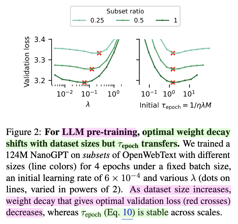
Intuitively, For example, if we use 1M sample for 1 epoch and bsz 100, we update param 10000 times. but if we train model with 100 times larger samples for each epoch, we will update parameter 100 times more, and for HP transferability (similar training dynamics) it seems to make sense to increase window size. and also, step size \(M\) is related to bsz, because if we increase bsz, \(M\) will be decreased, so we should increase weight decay to compensate this.
And for model size scale up, we know muP suggest \(1/n\) lr scaling rule for hidden matrix, so, we should scale weight decay like \(n \cdot \lambda\) to fix epoch time scale.
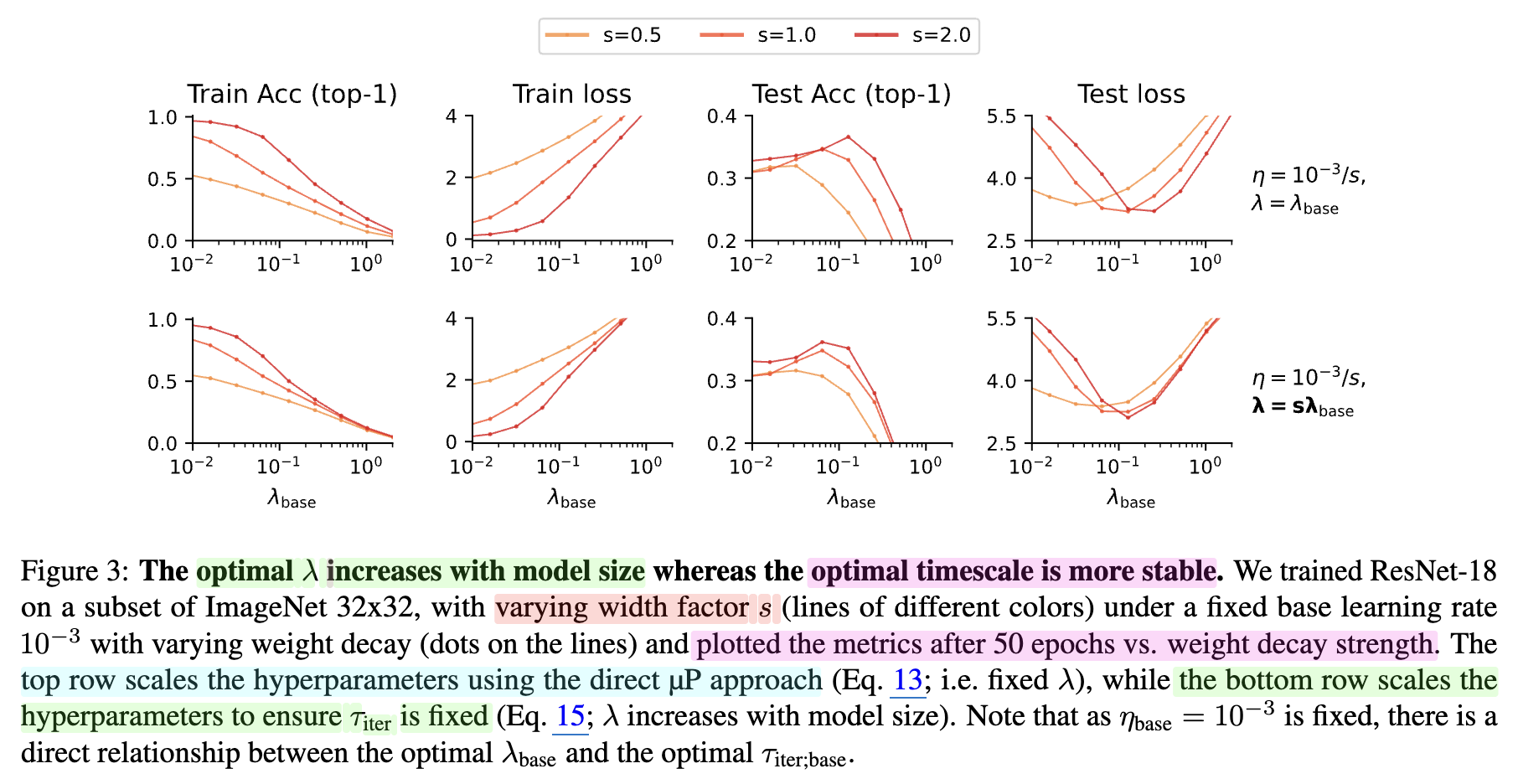
At this point, we don’t need to scale lr like \(\sqrt{bsz}\) for adamw as we increase bsz, rather we can conclude it could be better to control weight decay! Originally, \(\tau_{iter} = 1/(\eta \lambda)\) is \(1/\lambda\) if it’s truly decoupled weight decay, so in this case, we don’t need to scale weight decay according to model size. I guess this is another data point for why truly decoupled weight decay shows better transferability and performance.
Crebrase Team’s Power lines further investigate this and for largely overtrained regime, epoch time scale would not be fixed but decreased exponentially following power laws.
HP Scaling Laws
Though we can achieve HP transfer across training horizon by adjusting weight decay, it’s still complicated to predict because every factors like bsz, num tokens, adaptive optimizer’s HPs, … are all correlated. So, even though relying on empirical scaling laws may not feel mathematically beautiful, fitting power laws for HPs like lr or bsz given computing budget or training horizon seems reasonable in practice. Because Scaling Law is universal behavior.
To the best of my knowledge, DeepSeek was the first to empirically fit HP scaling laws for large-scale neural networks.
In DeepSeek LLM (DS-V1), they fit lr and bsz with respect to the compute budget \(C\):
How can we find this Scaling Law?
- Set optimzier (typicall adamw) with fixed beta 1,2 and eps
- For various values of \(N\) and \(D\), perform grid search.
- Plot near-optimal configurations (within 5% of the best validation loss).
- Fit a Power Law
| Source | attn type | FLOPs per token formula | calculated (FLOPs per “?” token) | changes | C vs LR | C vs Bsz (tokens per iter) |
|---|---|---|---|---|---|---|
| Kaplan et al | MHA | \(6N = 72 n_{layer} d_{model}^2\) | baseline | |||
| Hoffmann et al | MHA | \(72 n_{layer} d_{model}^2 + \underbrace{6 n_{vocab} d_{model}}_{logit}\) | +logit | |||
| DeepSeek V1 | MHA | \(72 n_{layer} d_{model}^2 + \underbrace{12 n_{layer} d_{model} l_{seq}}_{SDPA}\) | 4.3T per 2K tokens | +attn but only non-embedding | \(0.3318 C^{-0.1250}\) | \(0.2920 C^{0.3271}\) |
| DeepSeek-MoE 2B | MHA | (maybe same with DSV1) | 4.3T per 2K tokens | |||
| DeepSeek-MoE 16B | MHA | (maybe same with DSV1) | 74.4T per 4K tokens | |||
| Megatron-LM | MHA | \(\begin{aligned} & 72 n_{layer} d_{model}^2(1+\frac{l_{seq}}{6d_{model}}+\frac{n_{vocab}}{12 d_{model} l_{seq}}) & \\ & = 72 n_{layer} d_{model}^2 + \underbrace{12 n_{layer} d_{model} l_{seq}}_{SDPA} + \underbrace{6 n_{vocab} d_{model}}_{logit} & \\ \end{aligned}\) | +attn +logit | |||
| Minimax | MHA | \(72 n_{layer} d_{model}^2(1+\frac{l_{seq}}{6d_{model}}+\frac{5}{18{d_{model}}})\) | ||||
| Linear (Lightening) | \(72 n_{layer} d_{model}^2(1+\frac{1}{2 n_{head}}+\frac{5}{18{d_{model}}})\) | |||||
| Hybrid Linear (Lightening) | \(72 n_{layer} d_{model}^2(1+\frac{l_{seq}}{48d_{model}}+\frac{7}{16 n_{head}}+\frac{5}{18{d_{model}}})\) | |||||
| Moonlight | MLA | \(6N\) | \(0.0127 C^{-0.057}\) | \(0.0065 C^{0.4138}\) | ||
| Stepfun | GQA | \(6N\) | \(1.79 N^{-0.713} D^{0.307}\) | \(0.58 D^{0.571}\) |
- In the table:
- FLOPs/token does not reflect GQA (except for Minimax).
- Thoguh SDPA coefficient is 6 in theory (causal attn computes only upper triangle), but most of them use 12
If you’re unfamiliar with how FLOPs/token is computed, check Kaplan et al. (2020).
Briefly saying, for matrix multiply with \(X \in \mathbb{R}^{m \times n}, W \in \mathbb{R}^{n \times k}\), forward pass costs \(2mnk\) FLOPs (fused multiply-add; FMA), and backward roughly doubles this. Note that, Kaplan et al. considered attention didn’t contribute to C a lot in 2020 (if i remember correctly), But in 2025, with long contexts, attention terms become significant due to the quadratic sequence length term is not negligible anymore.
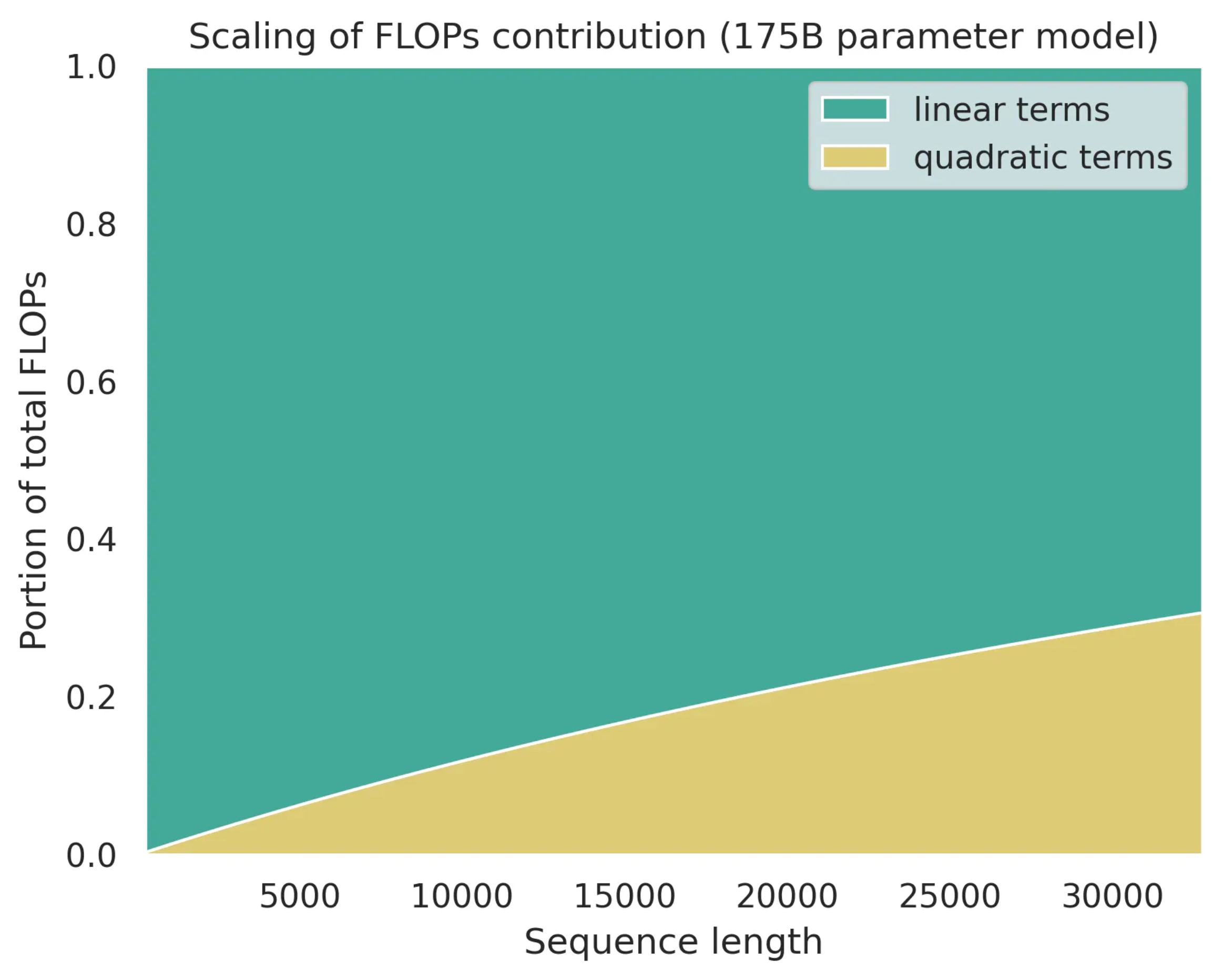 Fig. Source from Transformer FLOPs by Adam Casson
Even so, for GPT-4++-scale models (trillions of parameters), attention cost might again be negligible but i’m not sure what formula they used.
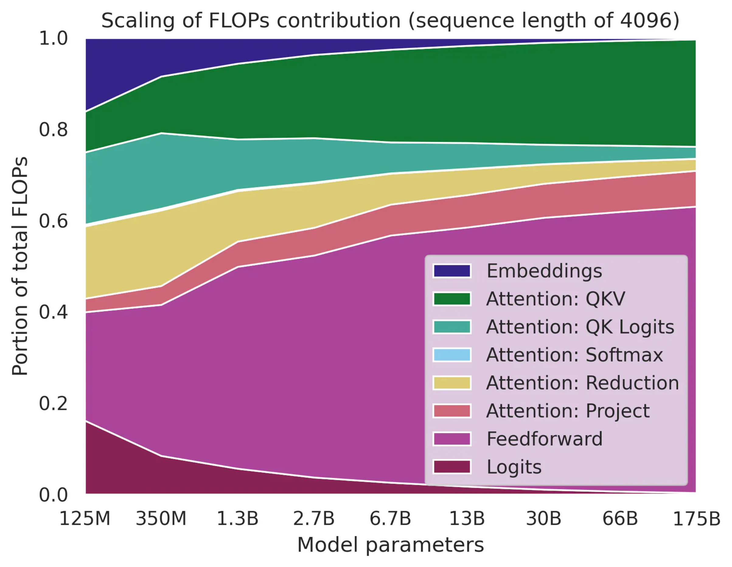 Fig. Source from Transformer FLOPs by Adam Casson
Among these, recently proposed Stepfun Law is especially interesting.
-
- Both optimal learning rate and batch size increase as dataset size grows.
- This makes intuitive sense: longer training = more variance, so we accumulate gradients with larger bsz. The rise in lr feels counterintuitive, but it’s a consequence of increased bsz i guess.
- Both optimal learning rate and batch size increase as dataset size grows.
-
- Optimal batch size is independent of model size.
- It seems counter-intuitive too because larger model perform better, and achievable loss is related to optimal and cbsz. However, it is not. (it is well-known, we will discuss this later in this post)
- Optimal batch size is independent of model size.
-
- Optimal lr follows left shift trend (as model size grows, it’s optimal lr should be downscaled)
- This aligns with muP little bit (in muP it follows a \(n^{-1}\)) but it does not match perfectly (maybe considering depth scaling)
- Optimal lr follows left shift trend (as model size grows, it’s optimal lr should be downscaled)
-
- Sparsity doesn’t affect the HP landscape.
- Whether the model is dense or MoE, if total parameters \(N\) are the same (not activated), the optimal HPs appear consistent.
- Sparsity doesn’t affect the HP landscape.
Finally, it is noteworthy that if you want to apply these scaling laws, you must match the training setup,
same lr scheduler and FLOPs/token formula.
Otherwise, predicted optimal values may diverge significantly.
 Fig. Stepfun Law shows how HP landscape shifts based on min lr and lr schedule.
About Terms like 'Optimal Batch Size' and 'Critical Batch Size'
Someone might think like “wtf is Optimal Batch Size?”. Indeed, bsz should not be tunable parameter for validation performance if you propetly set optimizer parameters like lr, adam beta 1,2 and eps. It should only be a factor for training efficiency (throughput).
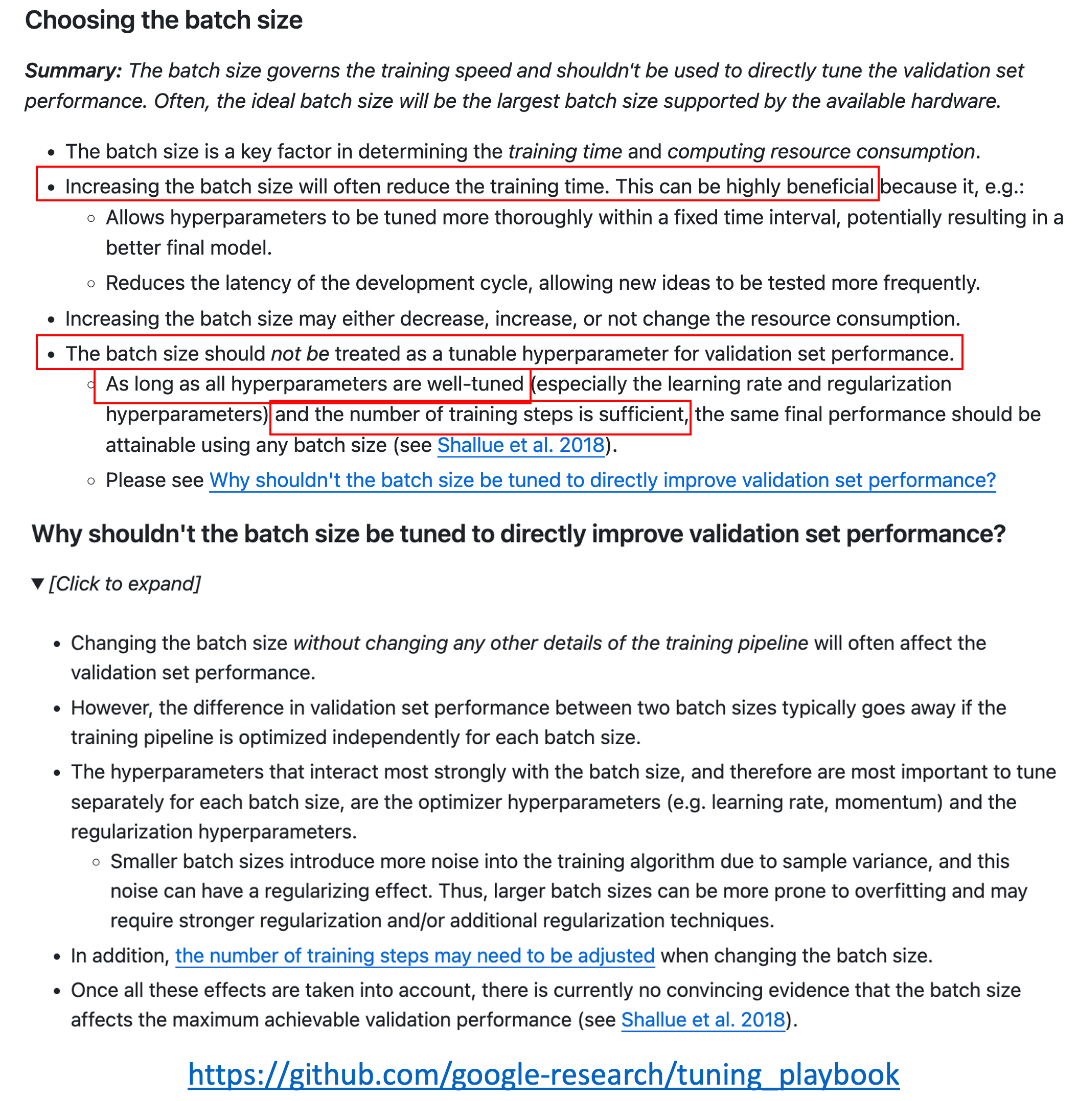 Fig. Source from Deep Learning Tuning Playbook
But bsz can’t be scaled up forever because there is a certain point called the Critical Batch Size (cbsz).

cbsz simply means “the point at which more parallelization (i.e., increasing bsz) becomes ineffective, because convergence still requires a minimum number of parameter updates (e.g., at least 1,000), since the gradient signal no longer improves.”
(Of course, you can check the original paper An Empirical Model of Large-Batch Training, but for simple intuition, here’s my thread about cbsz.)
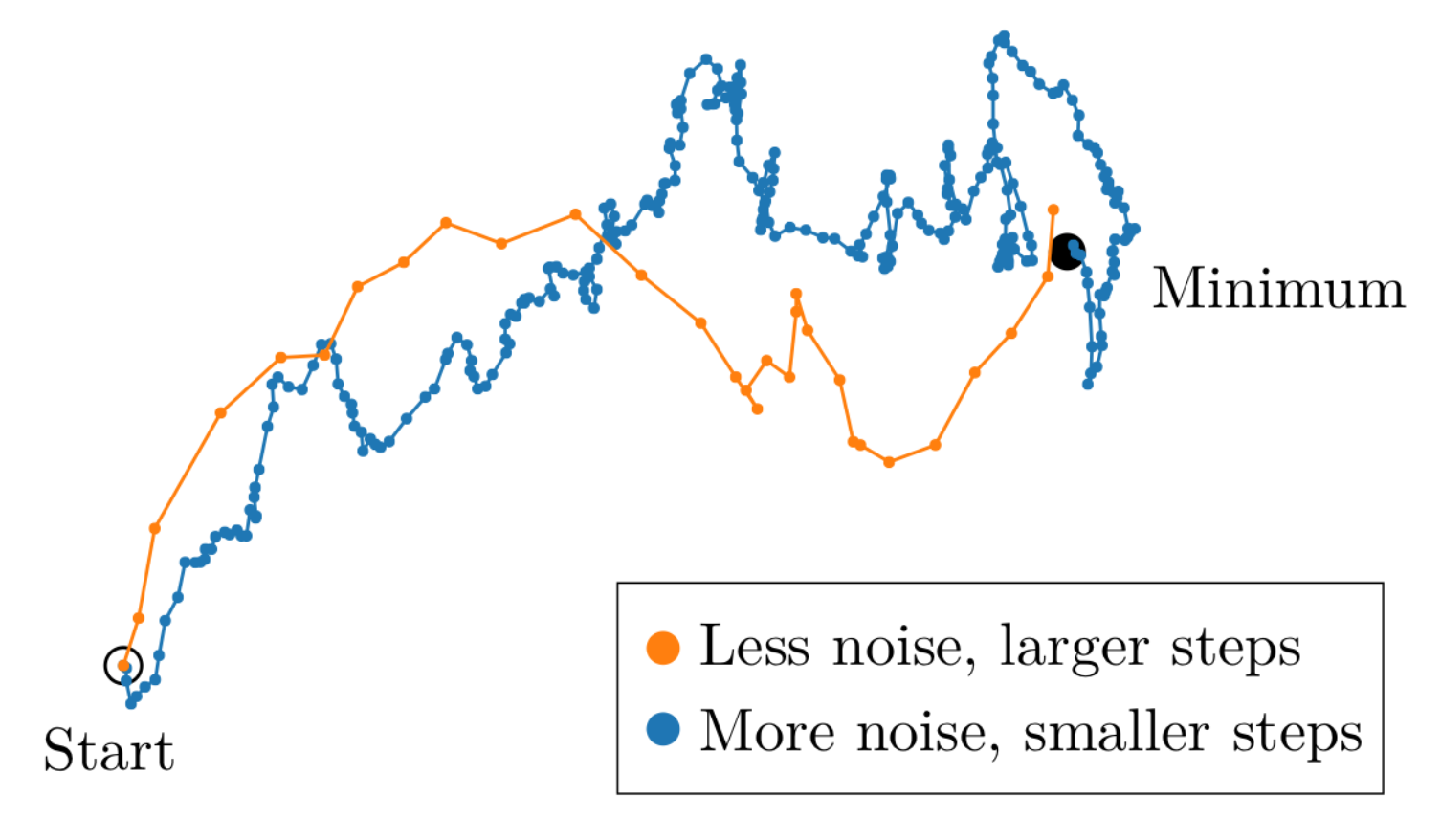 Fig. Less noisy gradient estimates allow SGD-type optimizers to take larger steps, leading to convergence in a smaller number of iterations.
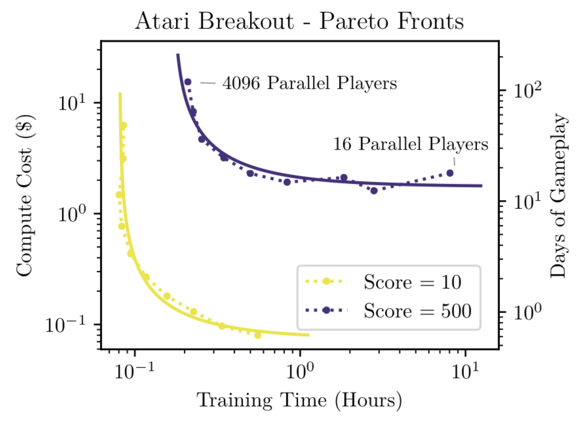 Fig. after certain point, compute cost for reaching same validation performance starts to be increased. before that, if you use 2x GPUs, bsz is doubled, and training time is reduced by 1/2, so it’s compute cost remain same.
So, as long as you don’t exceed the cbsz, model performance should not depend on bsz, and thus, an “optimal bsz shouldn’t really exist.
Additionally, when considering the generalization capacity of neural networks, things become a bit more complicated.
 Fig. Source tweet
So in most of cases, it’s safe to use smaller enough bsz unless you hurt MFU because there exists cbsz (ofc you should tune HPs for optimizer well). (In the Large Language Model (LLM) era, the concept of overfitting barely exists, we rarely apply dropout or similar regularization, and the generalization gap is often not a major concern.)
However, in real-world settings, there does exist an “optimal bsz”
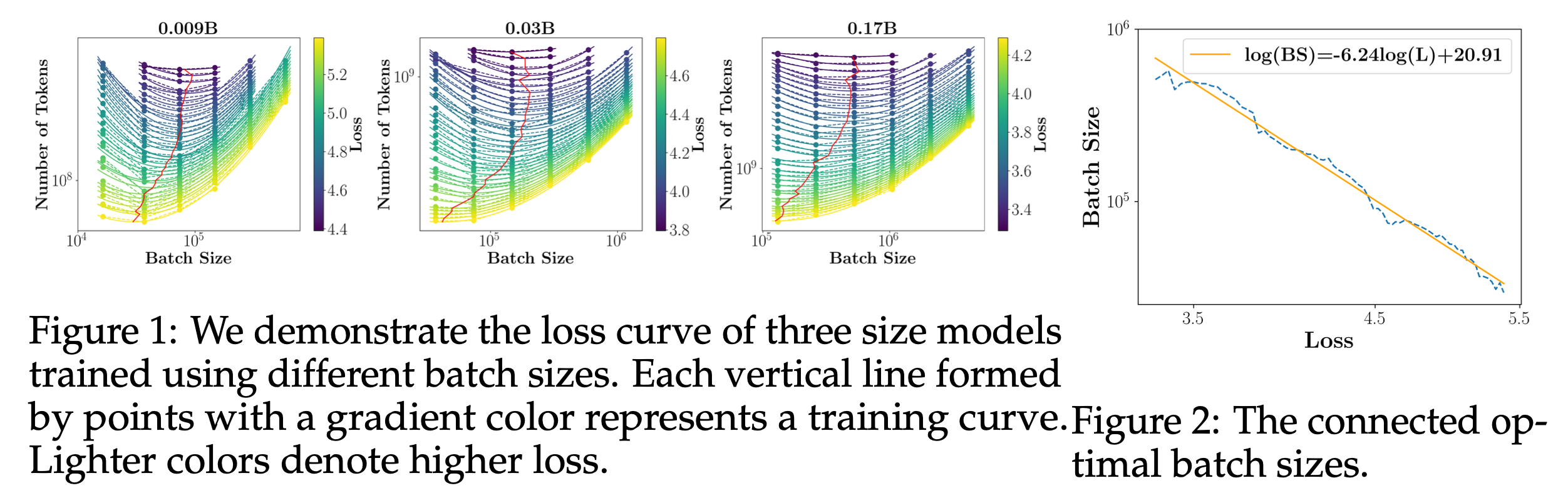 Fig. MiniCPM: Unveiling the Potential of Small Language Models with Scalable Training Strategies
Why?
I guess it’s because in real-world settings, we use stochastic optimizers, where the model is trained using sampled mini-batches, and we usually keep HPs like Adam(W)’s betas, epsilon, and weight decay fixed across different compute budgets, and only tune the lr.
In other words, if all HPs were tuned jointly (including Adam(W)’s betas, epsilon, weight decay, and lr), then the idea of an “optimal bsz” might be meaningless (see Simo’s note),
But in practice, as long as we only tune the lr while leaving the rest fixed, the notion of an optimal bsz still holds some practical value.
Fitted LR Scheudler for Real World LLMs
Anyway, we can fit scaling laws for HPs.
Below are actual lr scheduler examples derived from each paper’s HP scaling law.
The scheduler includes both the estimated peak lr and training steps (which relate to bsz),
so it’s helpful to compare how different their scaling laws are.
I tested all these methods using the DSV1 paper’s 7B and 67B model configurations with 2T tokens.
Most methods worked well ‘except for the StepFun law’.
According to StepFun, the model should be trained for much longer with a 2–3x larger peak lr, which doesn’t make sense to me.
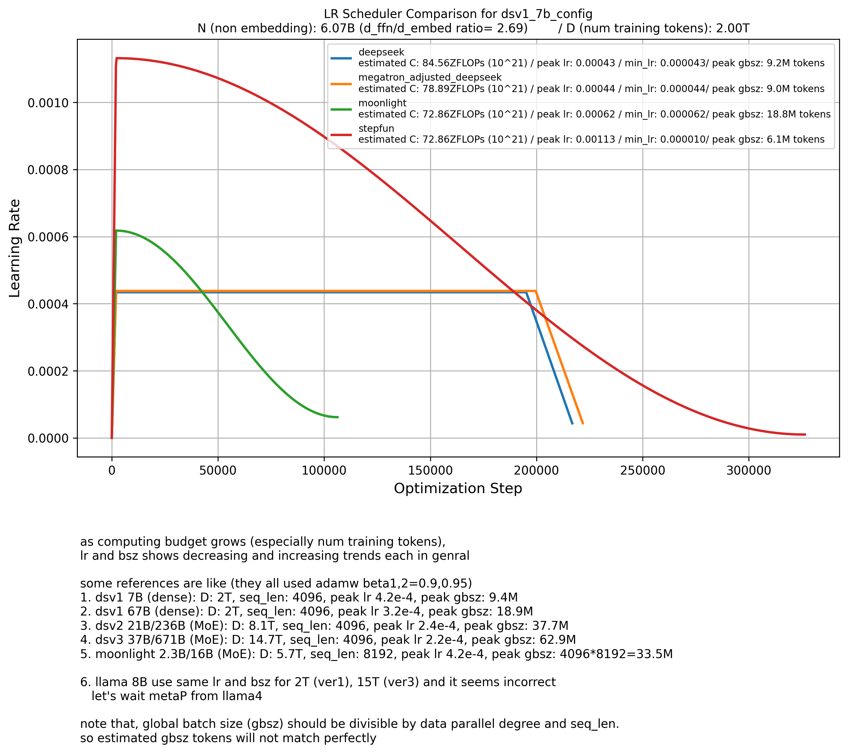
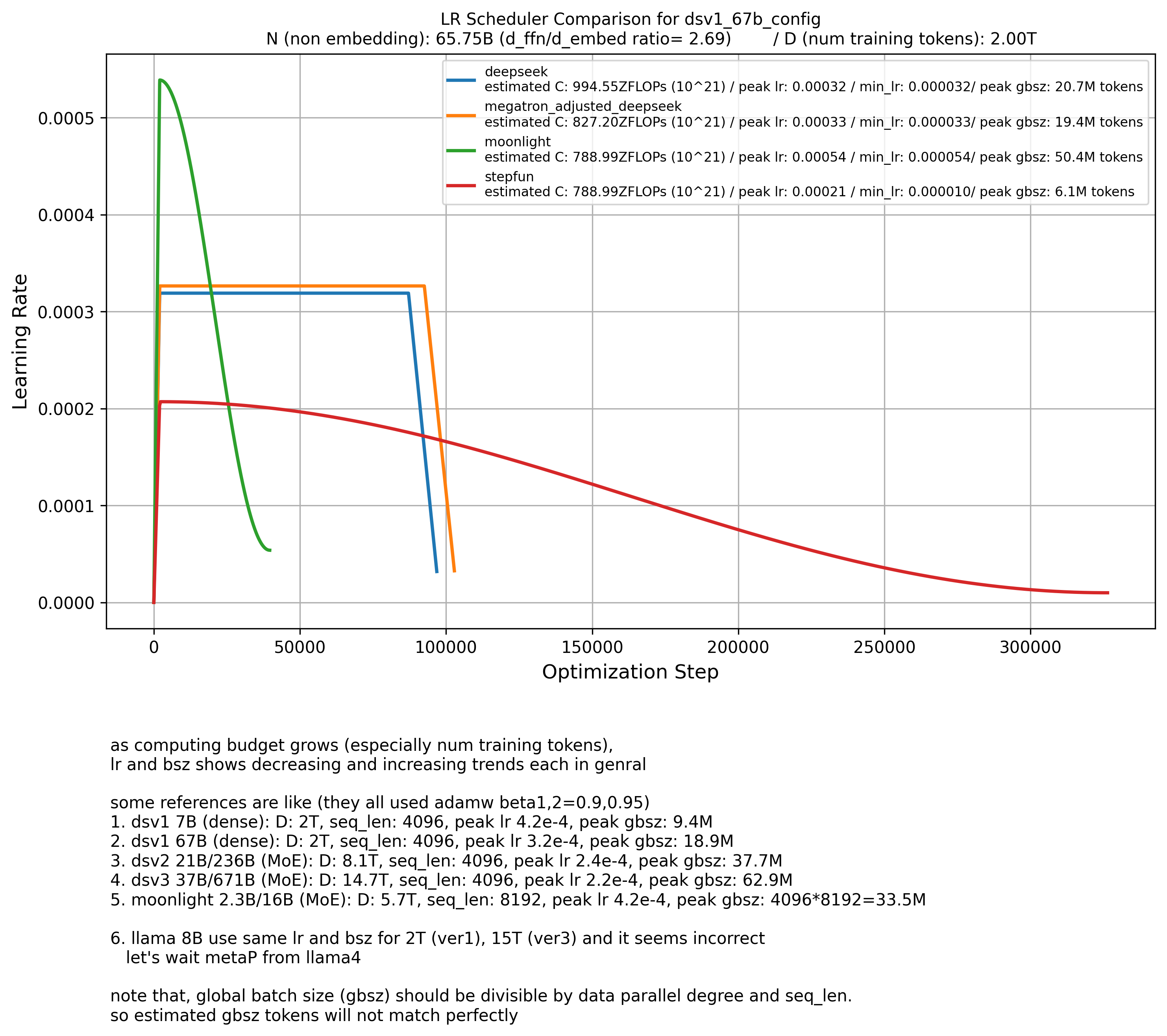
It makes sense that Moonlight’s peak LR is larger than DSV1’s,
because Moonlight used a cosine lr scheduler.
I also found that the rough estimate \(C = 6ND = (72 \cdot n_{\text{layer}} \cdot d_{\text{model}}^2) \cdot D\) (Kaplan-style compute formula) and DSV1’s FLOPs per token does not match with modern LLMs, especially wide and shallow models like Gemma-2 or MoE models.
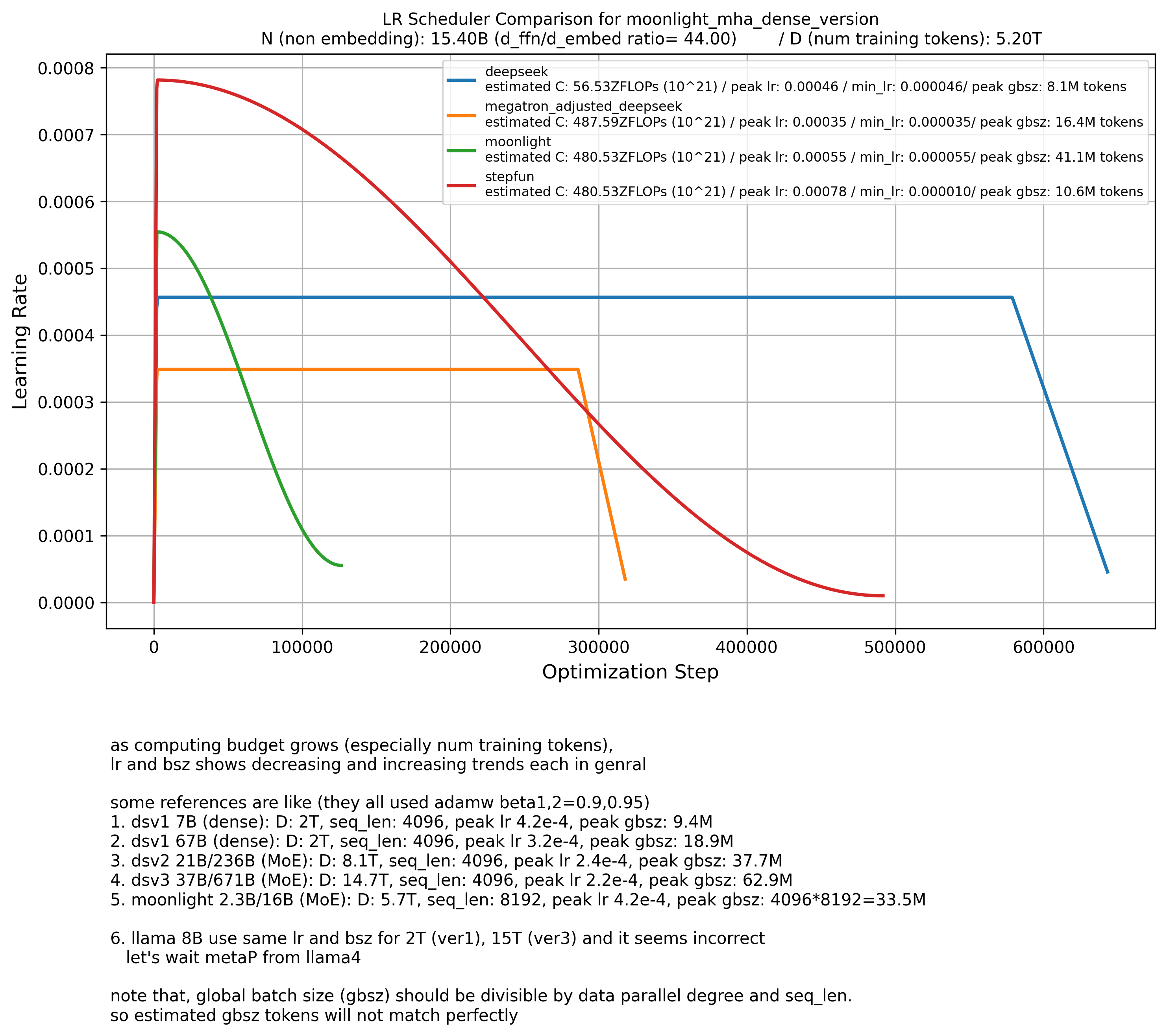
For MoE models, I assume \(N\) to be the total number of parameters, not just activated ones.
That’s because MoEs are essentially sparsely-activated versions of large dense models.
You can think of a 16B-parameter MoE with 2.3B activated as a 16B dense model where most weights are zero.
This is still valid even if you trained the full 16B model.
However, in this MoE model, the attention modules contribute very few parameters compared to FFNs.
That’s because MoEs typically scale up the FFN part.
For context: the FFN/attention ratio in models like LLaMA is around 3–4,
but Moonlight’s model has a ratio of 44,
and DSV1’s FLOPs-per-token calculation doesn’t account for this at all. (i’m not sure what scaling law they use for MoE models)
So, if you want to use any existing HP scaling law,
you should at least match the original setup they were derived from (e.g., wide/shallow ratio, LR scheduler, etc.).
Otherwise, you should fit your own law.
Some Scaling Behaviors of Critical Batch Size and Sensitivity to Optimizer
Originally, cbsz does not depend on model size, but rather on achievable loss.
So it makes sense to double the bsz once the model reaches a certain loss threshold in order to train faster.
This is called bsz warmup (or ramp-up).
In fact, MiniMax-01 was trained using this strategy.
They fit the cbsz scaling law, \(\text{cbsz} = f(L)\), and double the bsz following the fitted power law.
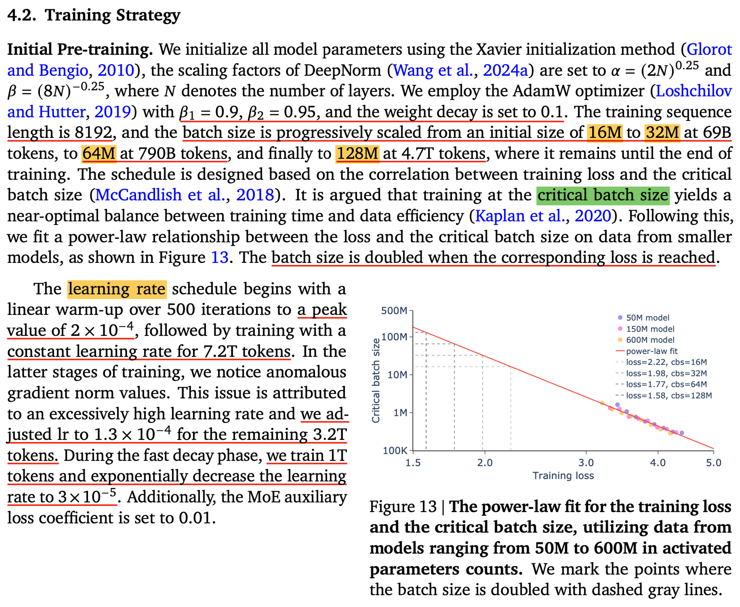 Fig. MiniMax-01: Scaling Foundation Models with Lightning Attention
However, achievable loss is also related to the compute budget \(C\), and \(C\) depends on both model size \(N\) and dataset size \(D\).
So one might intuitively think:
“Oh, if the model size increases, loss decreases (i.e., larger models are more sample-efficient),
so we can use a larger bsz for faster training.”
But that’s not true.
It has been shown that cbsz barely depends on model size, and that training tokens contribute much more.
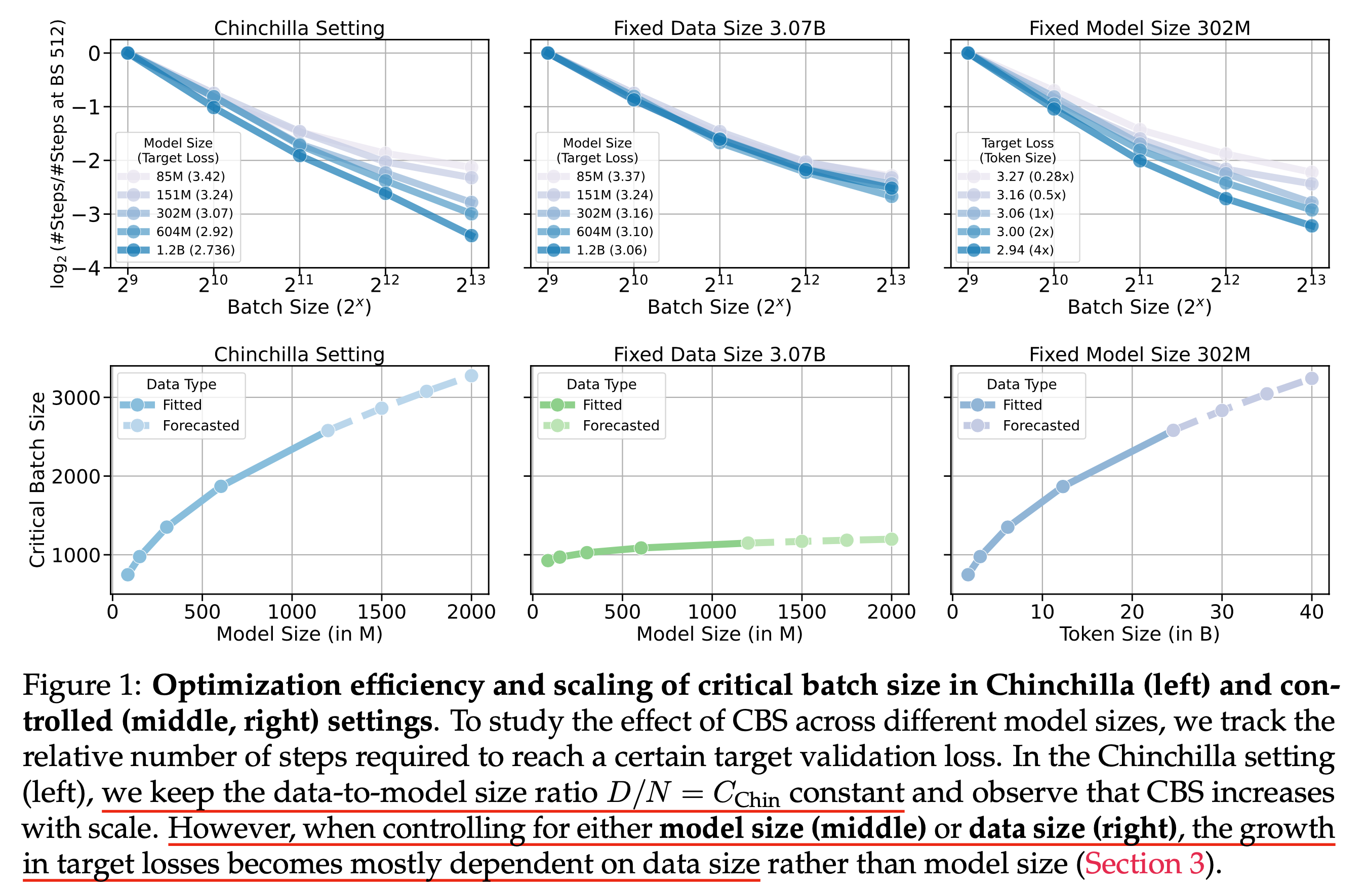 Fig. cbsz scaling behavior from How Does Critical Batch Size Scale in Pre-training?
(If you want to dive deeper, check out the full paper.)
It is noteworthy that cbsz is also sensitive to the optimizer.
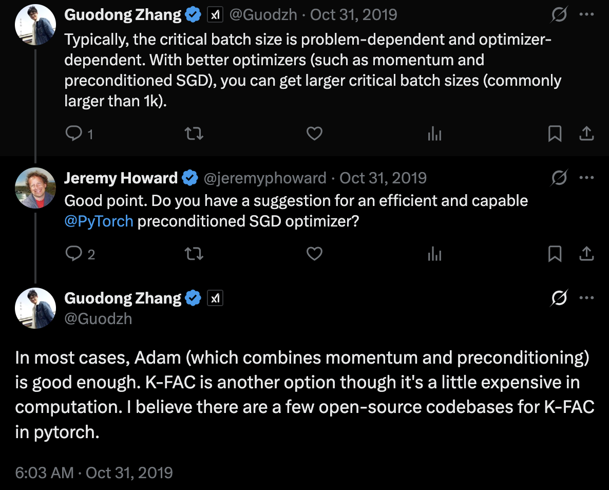 Fig. Source tweet
When we use Adam(W) for all experiments, cbsz is usually determined by data quality and training horizon. But if you use better optimizer, e.g. 2nd order optimizer like MomentUm Orthogonalized by Newton-Schulz (Muon), its cbsz is much larger, allowing us to train large transformers more efficiently. Here, “more efficiently” assumes an infinite-GPU scenario. For example, when using Adam(W), we can’t scale up bsz beyond 10M. So even with 50,000 GPUs, we can’t finish training faster, because we can’t update model parameters using 20M or 30M tokens. But if your cbsz threshold is 20M, you can reach the same validation loss with a 10M Adam(W) baseline twice as fast.
 Fig. Practical Efficiency of Muon for Pretraining
In Dion paper, they show that their new optimizer can be scaled even better than Muon for large-batch training.
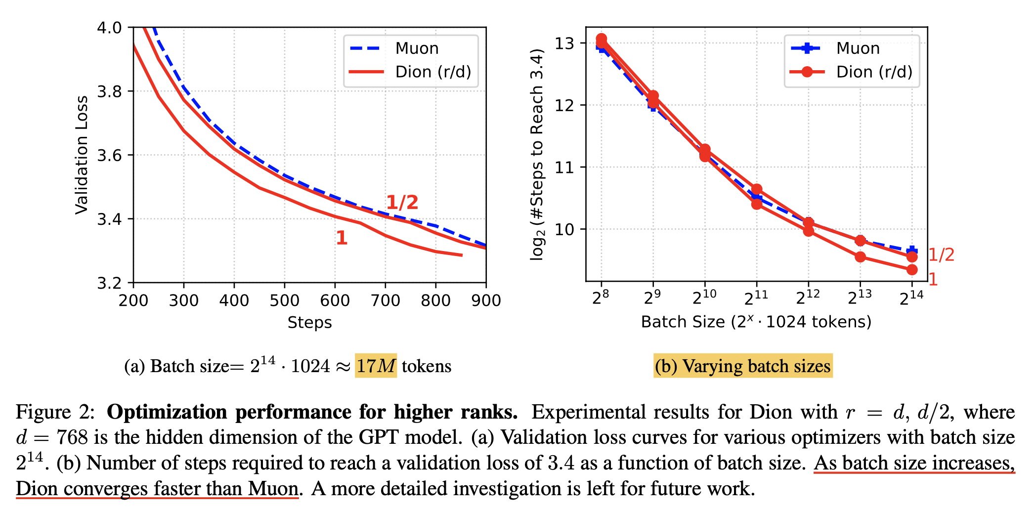 Fig. Dion: A Communication-Efficient Optimizer for Large Models
Pre-Training Hyperparameter References
Here are some reference bsz and lr used for LLM pre-training.
Note that I excluded papers that don’t explore or discuss scaling rules (at least in the paper).
For example, LLaMA 1, 2, and 3 all use the same bsz and lr, even though the number of training tokens varies from 2T to 15T,
and to me, that doesn’t make much sense.
So I decided to exclude them from this list.
| model | model type | activated param | total param | num. training tokens | bsz (tokens) | seqlen | lr | init std | optim | method used for predicting bsz, lr | notes |
|---|---|---|---|---|---|---|---|---|---|---|---|
| GPT-4 (Leaked, not sure) | MoE | 280B (E16K2S0) | 1.8T | 13T | 60M | 8K | ? | ? | ? | ? | (maybe muP is used) |
| DeepSeek-V1 7B | Dense | 7B | 7B | 2T | 9.4M | 4K | peak 4.2x10⁻⁴ (Warmup Constant) | 0.006 (SP) | adamw (0.9,0.95,0.1) | Scaling Law (from DSV1) | Multi Head Attention (MHA) |
| DeepSeek-V1 67B | Dense | 67B | 67B | 2T | 18.9M | 4K | peak 3.2x10⁻⁴ (Warmup Constant) | 0.006 (SP) | adamw (0.9,0.95,0.1) | Scaling Law (from DSV1) | Group Query Attention (GQA) |
| DeepSeek-MoE 2B | MoE | 0.24B (E64K6S2) | 1.89B | 2T | 4M | 2K | peak 1.08x10⁻³ (Warmup Constant) | 0.006 (SP) | adamw (0.9,0.95,0.1) | Scaling Law (from DSV1) | MHA |
| DeepSeek-MoE 16B | MoE | 2.8B (E64K6S2) | 16B | 2T | 18.4M | 4K | peak 4.2x10⁻⁴ (Warmup Constant) | 0.006 (SP) | adamw (0.9,0.95,0.1) | Scaling Law (from DSV1) | MHA |
| DeepSeek-V2 Lite 16B | MoE | 2.4B (E64K6S2) | 15.7B | 5.7T | 18.9M | 4K | peak 4.2x10⁻⁴ (Warmup Constant) | 0.006 (SP) | adamw (0.9,0.95,0.1) | Scaling Law (from DSV1) | Multi Head Latent Attention (MLA) |
| DeepSeek-V2 | MoE | 21B (E160K6S2) | 236B | 8.1T | 9.4M (init) -> 37.7M (at 225B) | 4K | peak 2.4x10⁻⁴ (Warmup Constant) | 0.006 (SP) | adamw (0.9,0.95,0.1) | Scaling Law (from DSV1) | MLA |
| DeepSeek-V3 | MoE | 37B (E256K8S1) | 671B | 14.8T | 12.6M (init) -> 62.9M (at 469B) | 4K | peak 2.2x10⁻⁴ (Warmup Constant) | 0.006 (SP) | adamw (0.9,0.95,0.1) | Scaling Law (from DSV1) | MLA, Multi Token Prediction (MTP) |
| MiniMax | MoE | 45.9B (E32K2S0) | 456B | 11.4T | 16M -> 32M (at 69B) -> 64M (at 790B) -> 128M (at 4.7T) | 8K | peak 2.4x10⁻⁴ (Warmup Stable Decay) | ? | adamw | Scaling Law for cbsz (it could be not optimal but efficient) | Hybrid Linear +Softmax Attention |
| Moonlight | MoE | 2.24B | 15.29B | 5.7T | 16.7M (33B) -> 33.5M (5.2T) | 8K | peak 4.2x10⁻⁴ (Warmup Cosine) | ? | adamw and muon | Scaling Law (from DSV1) | DSV3 style |
| MiniCPM 1.2B | Dense | 1.2B | 1.2B | 1.1T | 2M -> 4M | 4K | peak 0.01 (mu-transfered, Warmup Stable Decay) | 0.1 (muP) | ? | muP and Scaling Law for bsz | |
| MiniCPM 2.4B | Dense | 2.4B | 2.4B | 1.1T | 4M | 4K | peak 0.01 (mu-transfered, Warmup Stable Decay) | 0.1 (muP) | ? | muP and Scaling Law for bsz | |
| Granite 3.0 | MoE | 800M | 3B | 10T | 4M | 4K | peak 0.02 (mu-transfered, Power Scheduler) | ? | ? | muP | |
| Hunyuan-Large | MoE | 52B (E16K1S1) | 389B | 7T | ? | ? | ? | ? | ? | ? | Cross Linear Attention (CLA) |
QK Layernorm and "Put Everywhere Norm"
Recently, many researchers have started placing LayerNorms everywhere, including:
- After the Q and K projections
- Before residual additions (Swin-v2, Chameleon, Gemma-2,3 and OLMo-2)
- Mixing post-norm and pre-norm configurations (Mix-LN)
- …
 Fig. Source from Methods of improving LLM training stability
They seem to work because they keep the range of pre-activations and gradients within a reasonable bound. (However, they may still fail to address extremely large activations as expected. For example, in Gemma-3, residual post-norm and softcapping fail to suppress excessively large activation norms)
One of the earliest and most prominent “put-everywhere norm” techniques, QK-LayerNorm, comes from Scaling Vision Transformers to 22 Billion Parameters, where it works well.
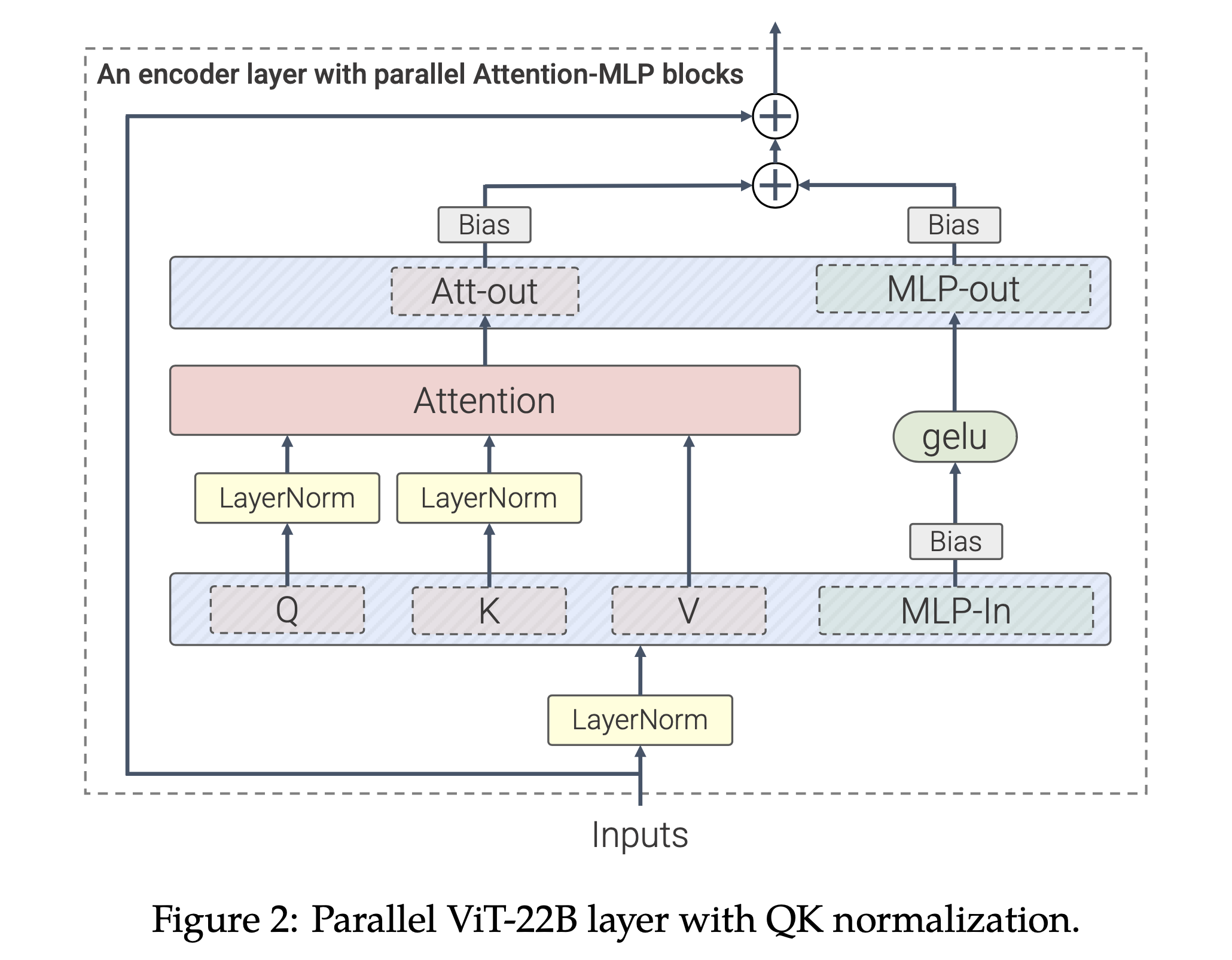
The key observation of this paper is that the L2 norm of logits before softmax (before Scaled Dot Product Attention (SDPA) and output head) is critical to prevent loss divergence.
So they normalize some tensors to ensure logits don’t blow up, and it worked.
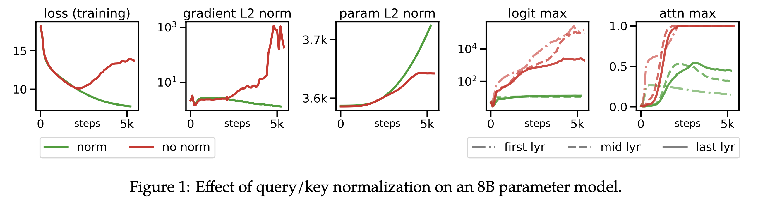
This idea was further studied in Small-scale Proxies for Large-scale Transformer Training Instabilities,
where the authors report that QK-LayerNorm enlarges the lr basin. This means lr sensitivity is reduced, making it easier to find near-optimal performance across a range of model widths.
And, this is compatible with muP. Of course, some may ask:
“Why should we use with QK-LayerNorm when muP already enables hyperparameter transfer? And, it could reduce throughput due to increased kernel launch overhead.”
That’s a valid point, but as we discussed earlier, muP doesn’t guarantee HP transfer across training horizon or bsz. So using QK-LayerNorm can be a good practical choice because it can increase the probability of choosing near-optimal lr.
In addition, it has been shown to outperform the vanilla Transformer even in settings where the HPs are optimal.
And it seems that all these “put-everywhere norm” enlarge lr basin empirically.
 Fig. Source from Methods of improving LLM training stability
+Updated) However, even QK-LayerNorm can be problematic, as it may reduce the model’s ability to handle long contexts by suppressing the sharpness of the attention logits. This means the model may fail to assign sufficiently high probabilities to target tokens, especially as the number of classes increases. (We might need to consider proper parameterization or architectural improvements instead of relying on naive QK-LayerNorm)
 Fig.
Fig.
Updated) Relationship between Muon and muP
Thoguh there is good literatures such as Jeremy’s blog post andLaker’s blog post (they are both authors of Muon), i’d like to cover Muon optimizer bit. Recently, Muon (MomentUm Orthogonalized by Newton-Schulz) has been very popular optimizer, but it’s still looks complicated for newcomers.
Why it works? What’s the relationship between Muon and muP? (It contains Mu-on)? does it ensure HP transfer?
One can explian because Adaptive optimizers like Adam(W) produce parameter update tensor with low stable rank, so there is few chance to explore large space of model, and Muon resolve this by boosting other directions with low eigenvalues.
That’s good point, but one thing we should keep in mind is that, Muon can be dervied A Spectral Condition for Feature Learning which is used for deriving muP. Indeed, Muon with spectral muP (name is bit different with pure muP, but it’s same) also ensure maximal update itself, and it can transfer HP such as lr.
Key summary of Muon is as follows.
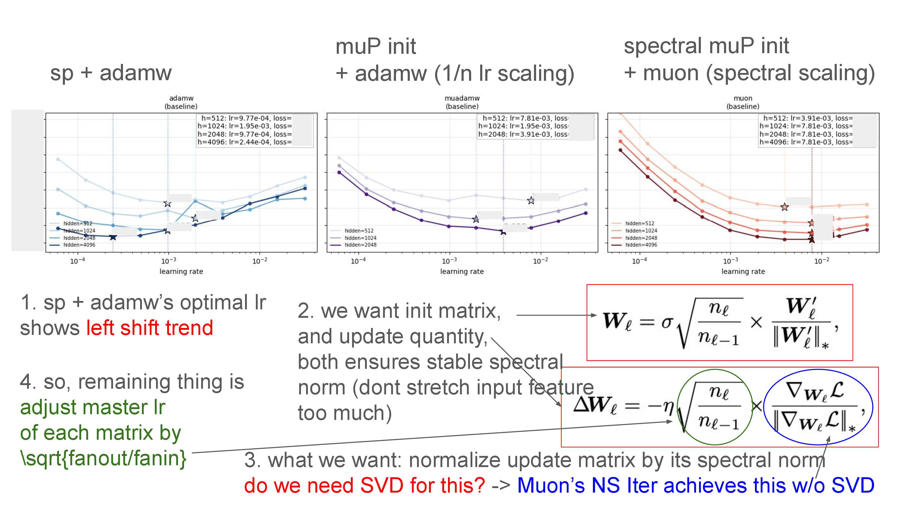 Fig. Source tweet
Indeed, the motivation of Muon is same as muP. What we want here is that, we don’t want every layer’s output (pre-)activation don’t blow up as we scale (we define this by big Theta notation before).
\[\left\| \boldsymbol{h}_{\ell} \right\|_{2} = \Theta(\sqrt{n_{\ell}}) \text{ and } \left\| \Delta \boldsymbol{h}_{\ell} \right\|_{2} = \Theta(\sqrt{n_{\ell}}), \text{ at layers } \ell = 1, \dots, L-1.\]And for this, we want to ensure not only initialized weight parameters’ spectral norm become stable, but also our update quantities’ spectral norm become stable.
\[\left\| \mathbf{W}_\ell \right\|_* = \Theta \left( \sqrt{\frac{n_\ell}{n_{\ell-1}}} \right) \text{ and } \left\| \Delta \mathbf{W}_\ell \right\|_* = \Theta \left( \sqrt{\frac{n_\ell}{n_{\ell-1}}} \right), \text{ at layers } \ell=1, \dots, L.\]Because as we discussed before (in muP section), optimization process indeed accumulations of parmaters and the gradients which is (post-)processed by our optimizers like Adam.
\[\mathbf{h}_{\ell}(x) = \mathbf{W}_{\ell}\mathbf{h}_{\ell-1}(x) \quad \text{for } \ell = 2, \dots, L.\] \[\mathbf{h}_{\ell}(\mathbf{x}) + \Delta \mathbf{h}_{\ell}(\mathbf{x}) = (\mathbf{W}_{\ell} + \Delta \mathbf{W}_{\ell})(\mathbf{h}_{\ell-1}(\mathbf{x}) + \Delta \mathbf{h}_{\ell-1}(\mathbf{x})).\]But why spectral norm matters? What really matters here is we don't want our model's activations blow up as forward propagation through many layers, also throughout the entire optimization procedure, and what we should control to achieve this here is how much each layer's weight matrix can stretch input feature and it’s actually spectral norm. And spectral norm is same as largest singular value of given matrix (matmul is actually rotation -> stretch -> rotation, and stretch is very important).
To achieve this, we can force spectral norm of our initialized weight and update quantity using SVD. Because we can set all singular values (Simga matrix) as 1 after SVD. Intialization seems easy because no matter how SVD is heavy operation, we can just apply SVD to random matrices once at init point, but applying SVD for update quantity every iteration is non-sense.
\[\mathbf{W}_\ell = \sigma \sqrt{\frac{n_\ell}{n_{\ell-1}}} \times \frac{\mathbf{W}'_\ell}{\| \mathbf{W}'_\ell \|_*},\] \[\Delta \mathbf{W}_\ell = -\eta \sqrt{\frac{n_\ell}{n_{\ell-1}}} \times \frac{\nabla \mathbf{w}_\ell \mathcal{L}}{\left\|\nabla \mathbf{w}_\ell \mathcal{L}\right\|_*},\]At this point, we can use Newton Schulz (NS) Iteration to make every singluar values of update quantiy’s to be 1. This is very clever choice because NS Iteration is done by 5 times matmul which can leverage modern GPGPU’s tensor cores unlike SVD. (once again, see the below figure’s formula)
Actually, we can (spectral) muP controls this spectral norm of update quantity by adjusting Adam(W)’s lr by 1/n (n is width), but Muon directly achieve this more natually. So, as you can see, spectral muP init + Muon can give us not only good performance but also good HP transfer across model width.
Some Tips for Training Large Transformers
(This subsection might be slightly outdated as it is based on my personal notes from early 2024.)
- Use
bfloat16 (bf16)instead offloat16 (fp16)- It has the same dynamic range as
float32 (fp32)and doesn’t require dynamic loss scaling (no overhead). - Update) consider
fp8orfp4if you have state-of-the-art accelerators and no skill issues.
- It has the same dynamic range as
-
Consider using
Maximal Update Parameterization (muP)instead of Standard Parameterization (SP) - Monitor logits and norm or RMS of all (pre-)activations
- Training instability typically arises in logits (values before the softmax operation)
→ See Small-scale proxies for large-scale Transformer training instabilities- Attention logits: Use QK LayerNorm – may incur additional compute overhead.
- Output logits: Use Z-loss – also adds computational cost.
- Recently, Gemma 2 introduced attention logit soft-capping for improved stability (also used by Grok).
- Pre-activations should not explode as model width grows.
- Some discrepancy is okay, but if your output’s L2 norm becomes much larger than your small-scale proxy, it’s red flag.
- Training instability typically arises in logits (values before the softmax operation)


- Remove bias terms in linear layers
- Most frontier LLMs do not use bias in their linear layers, even recent state-of-the-art models.
- Likely due to numerical stability and better generalization.
- For numerical stability, I’ve seen cases where bias terms were so large that log-prob ratio for PPO (e.g. with vLLM inference) diverged at step 0. (It should ideally be 0.)
- And, well, bias is literally bias. You’d better off tuning your slope (weight), not your bias for model generalization (i guess).
- However, Qwen2 uses bias in QKV projection, based on Su Jianlin’s blog post, claiming it helps generalization for long context.
- Likely due to numerical stability and better generalization.
- Most frontier LLMs do not use bias in their linear layers, even recent state-of-the-art models.
- Reconsider your optimizer HPs
- The standard setup for training large-scale transformers is often \((\beta_1, \beta_2, \epsilon) = (0.9, 0.95, 1e{-8})\),
but these defaults are not guaranteed to be optimal. - If you use gradient clipping, 1.0 is a common, but who knows it’s optimal.
- The standard setup for training large-scale transformers is often \((\beta_1, \beta_2, \epsilon) = (0.9, 0.95, 1e{-8})\),
- Vanilla LayerNorm vs RMSNorm
- RMSNorm is faster in terms of both convergence and throughput.
- Never cross the Critical Batch Size (cbsz)
- we discussed this a lot in this post
- Always track Machine FLOPs Utilization (MFU)
- MFU means “how many FLOPs do you utilize in a second”. you should track MFU and if it’s lower than 55% (in general case, e.g. 128~256 ampere GPUs, bf16), there might be bottleneck somewhere for example
- Your algorithm is not scalable
- Your distributed setup is inefficient:
- FSDP ring latency too high
- Too much tensor parallelism (TP)
- Excessive gradient checkpointing
- CPU offloading is not fully overlapped
- …
- MFU means “how many FLOPs do you utilize in a second”. you should track MFU and if it’s lower than 55% (in general case, e.g. 128~256 ampere GPUs, bf16), there might be bottleneck somewhere for example
- About QK LayerNorm
- I’d like to say
"Don't get too caught up in finding completely optimal HPs". IMO, it’s ok to use near-optimal HPs, so youd better use your resource to data quality. - As we discussed above, it’s not silver bullet especially in long context regime.
- I’d like to say
Let me tell about “why should we care MFU” little bit. It is noteworthy that the one of the most important thing when scale up is "if your method (new arch, new learning algorithm) is scalable or not". If your method improves convergence speed by 10%,
but reduces throughput by 20%, is it really an improvement?
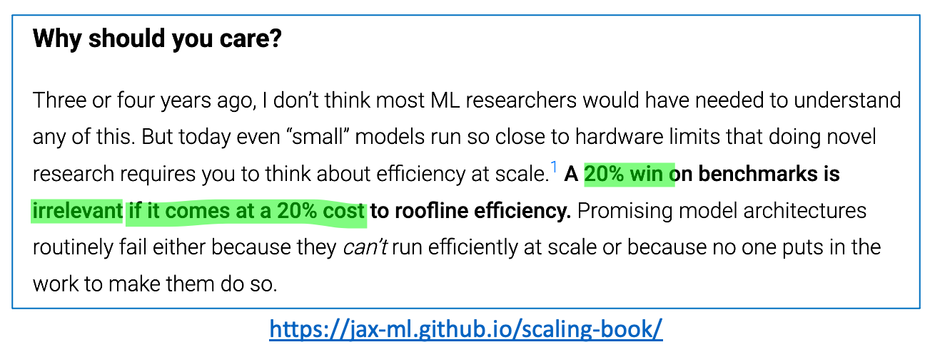 Fig. How to Scale Your Model from Jacob et al.
There are some examples like:
- Multi-Head Latent Attention (MLA)
- Requires more memory and I/O than vanilla MHA or GQA
- Needs fused up_proj + RoPE + norm + flash + selective checkpointing
- “Put norm everywhere”
- Increases kernel launch overhead, I/O
- You may need fused linear+norm kernels (in small-scale, it’s negligible i guess but)
- Shampoo or Muon optimizers
- Require gathering sharded weight matrices to compute statistics
- Communication and computation must be well overlapped
A good training algorithm (and infra design) should scale well with both model size and hardware.
Tuning Adam beta 1,2 could be non-trivial
It is well known that adam(w) beta1,2,eps=(0.9,0.95,1e-8) works well. But it could be not optimal. I didnt explore this topic a lot, but How Does Critical Batch Size Scale in Pre-training? present some analysis, so i recommend you to read this paper.
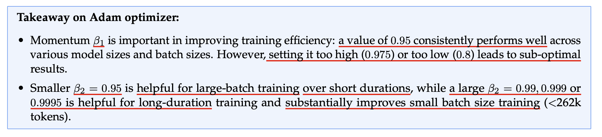 Fig. Adam beta 1, 2 ablation from How Does Critical Batch Size Scale in Pre-training?
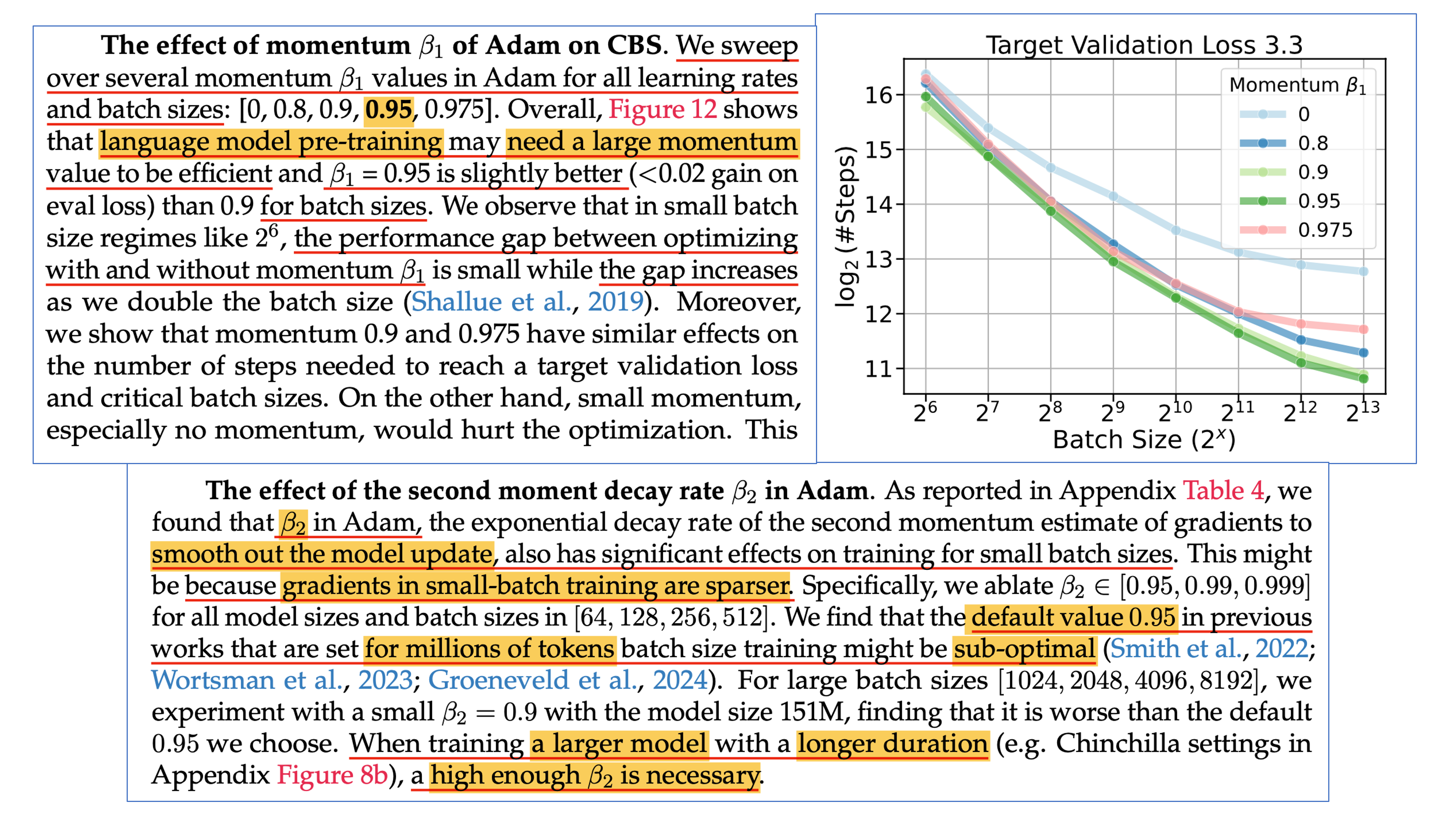 Fig. Adam beta 1, 2 ablation from How Does Critical Batch Size Scale in Pre-training?
About 0.02 and 0.006 init std
It’s noteworthy that some open-source framework model configs hardcode std=0.02, a value inherited from GPT-2 (up to 1.5B scale).
However, it’s not suitable for larger models like 30B, 60B, etc., because 0.02 roughly corresponds to \(\sqrt{1/1536}\), the standard deviation derived from SP’s fan-in variance.
It’s also questionable to use the same 0.02 for FFN modules, where the inner dimension is typically 3–4× larger than the attention embedding dimension.
>>> for d in range(512,8192+512,512):
...     print(f"d_model (width): {d}, 1/sqrt(width): {1/math.sqrt(d):.4f}")
...
d_model (width): 512, 1/sqrt(width): 0.0442
d_model (width): 1024, 1/sqrt(width): 0.0312
d_model (width): 1536, 1/sqrt(width): 0.0255
d_model (width): 2048, 1/sqrt(width): 0.0221
d_model (width): 2560, 1/sqrt(width): 0.0198
d_model (width): 3072, 1/sqrt(width): 0.0180
d_model (width): 3584, 1/sqrt(width): 0.0167
d_model (width): 4096, 1/sqrt(width): 0.0156
d_model (width): 4608, 1/sqrt(width): 0.0147
d_model (width): 5120, 1/sqrt(width): 0.0140
d_model (width): 5632, 1/sqrt(width): 0.0133
d_model (width): 6144, 1/sqrt(width): 0.0128
d_model (width): 6656, 1/sqrt(width): 0.0123
d_model (width): 7168, 1/sqrt(width): 0.0118
d_model (width): 7680, 1/sqrt(width): 0.0114
d_model (width): 8192, 1/sqrt(width): 0.0110
But you can still train your model successfully without deep mathematical justification.
According to Using DeepSpeed and Megatron to Train Megatron-Turing NLG 530B,
they use lower init std than SP, like \(1/\sqrt{3 \cdot \text{fan-in}}\).
And DeepSeek consistently uses 0.006 as the init std from v1 (7B dense) to v3 (671B total MoE).
I honestly don’t know exactly why this works so well.
My guess is that it’s due to the combination of many normalization modules, residual connections, and adaptive optimizers, but who really knows?
Rethinking Conventional Wisdom
Inspired by Rethinking Conventional Wisdom in Machine Learning: From Generalization to Scaling. In conventional regime, small bsz and lr at Edge of Stability (EoS) is known as good choice, but it does not seem to fit in large scale training and overparameterized regime. So, i’d like to recommed you to doubt conventional wisdom when scaling up NN.
 Fig. lr at EoS is not optimal in Large Scale Regime
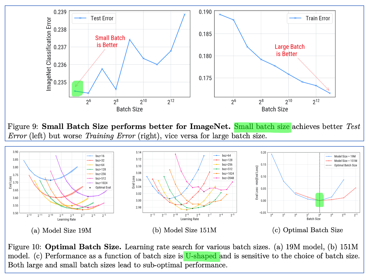 Fig. smaller batch size is not optimal in Large Scale Regime
Outro
-
Is pre-training scaling done?- Ilya said pre-training is done (of course, only for frontier labs lol).
- Team OpenAI admitted that before 2024–25, compute was the bottleneck, but now the bottleneck is dataset availability.
I guess frontier labs have already used up the entire internet.
-
However, there is still room for scaling IMO- Better optimizer
- GDM, moonshot ai, and … show that 2nd optimizer is promising
- GDM uses Shampoo for distillation, but idk they use this for pre-training or not
- we can make our model learn more features using same amount of sequences (better sample efficiency)
- xAI’s researcher, Guodong Zhang confirmed they don’t use adam and need more
- Recently, OpenAI hired the creator of Muon, Keller Jordan
- GDM, moonshot ai, and … show that 2nd optimizer is promising
- Better architecture
- more scalable architecture
- sparse model like MoE is already used for many frontier models but we need more
- more scalable arch for long context
- native sparse attention, …
- more scalable architecture
- Multimodal
- frontier models are already native multimodal but there are still many video and speech, … data and they have much richer information than texts
- Better optimizer
Transformer was a revolution level improvement, but it seems not enough today. I believe we can keep pushing the limit by improving architecture and optimizer.
 Fig. from my past slide on Scaling Law and MoE
 Fig. from my past slide on Scaling Law and MoE
 Fig. from my past slide on Scaling Law and MoE
Western frontier labs have been studying MoE for a long time,
and Chinese labs are following the trend. Recently, State Space Models (SSMs), hybrid attention, and sparse attention models have been activly studied, and we should know how to scale these models (ofc these models also consists of bunch of matmul, but)
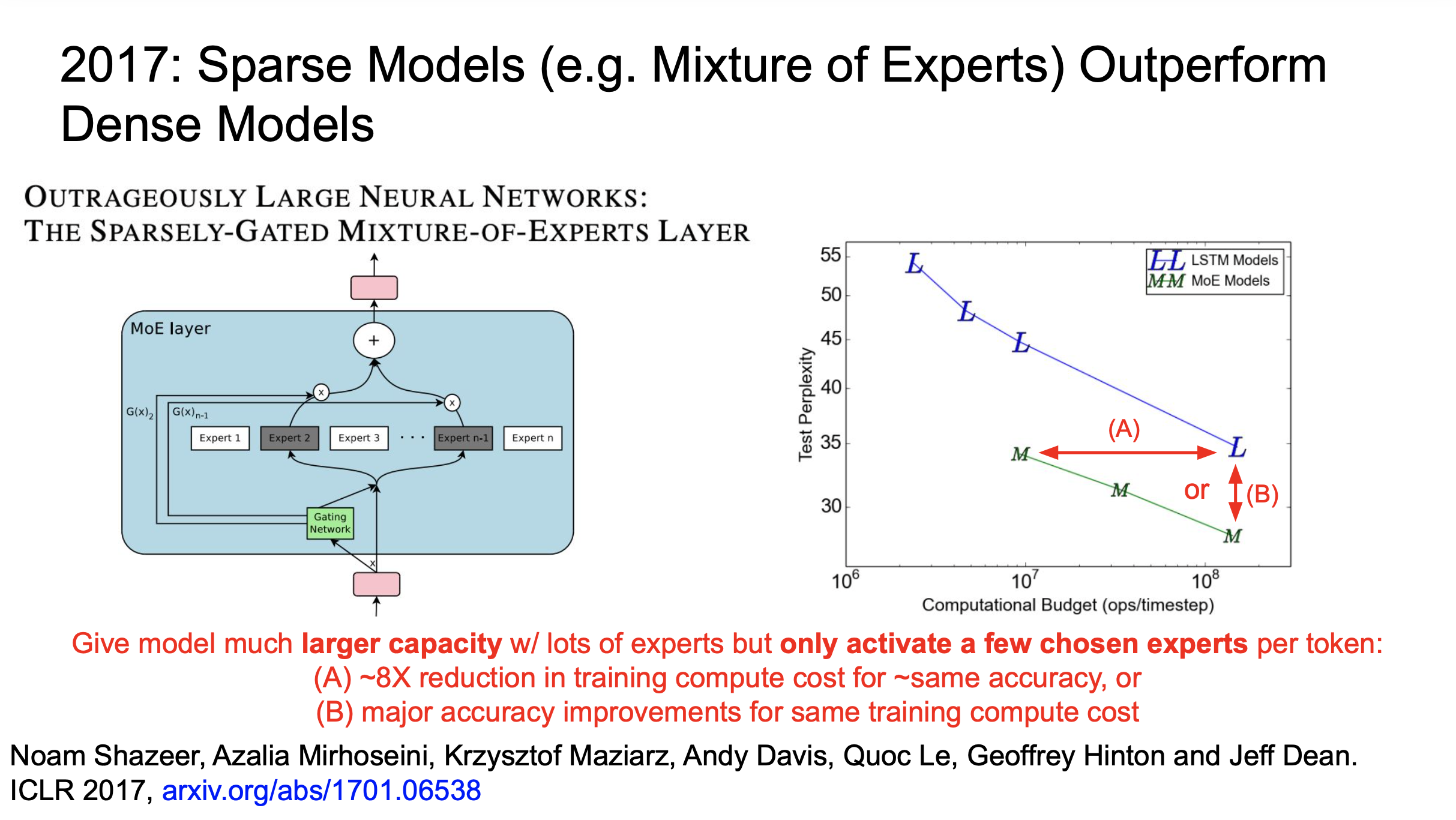 Fig. from Jeff Dean’s Talk
 Fig. from Jeff Dean’s Talk
Though it is well known that techniques like MoE and second-order optimizers work well, there hasn’t been much public discussion on how to properly parameterize them for scaling.
- e.g. does muP still work for MoE, muon, shampoo or something?
- Updated) Muon is maximal update itself and can ensure HP transfer with spectral muP init.
Acknowledgement
I’d like to thank everyone for taking the time to read this post and for sharing any insightful feedback. Special thanks to Simo Ryu for many thoughtful discussions, Jingyuan Liu for sharing the reasoning behind MoE scaling factors, Alexandre for the experimental results on Mamba with muP. And I’d also like to thank Seonghyeon Kim, Charlie Blake, and Donghoon Ham for their warm encouragement and helpful feedback.
- Updated) i’d like to say thank you to Xi Wang for helpful discussion for scaling training horizon (dataset size).
References
- Key Papers
- Videos
- Edward Hu - μTransfer: Tuning GPT-3 HPs on one GPU, Explained by the creator
- Greg Yang - Feature Learning in Infinite-Width Neural Networks
- Greg Yang - Tuning Large Neural Networks via Zero-Shot Hyperparameter Transfer
- Large N Limits: Random Matrices & Neural Networks from Greg Yang w/ Timothy Nguyen
- Katie Everett - Scaling Exponents Across Parameterizations and Optimizers
- Others